Interface - ESDC
Interface Description
ESASky is an exploration style interface where the entire sky is available to search and explore. Its functionalities are described below:
- ESASky modes and basic exploration functionalities
- Search field
- Skies menu
- Data panel (Imaging, Catalogue and Spectra search)
- Solar System Objects search
- Multi-messenger events
- Scientific Publications search
- External Data Centre search
- Target list feature
- Observations Planning tool
- ESA/Hubble Outreach Images
- ESA/Webb Outreach Images
- Euclid Outreach Images
- Snapshot feature
- Selection tool
- Explore random targets feature
- Bookmark / sharing feature
- Additional information and help menus
- Save an ESASky session
- User area

esasky modes and basic exploration functionalities
New to version 3.0, you can select the mode in which you want to work: Science mode or Explorer Mode. This can be done in the welcome dialog window or with the switch on the top bar:
Science mode includes all access to science ready data, skies, publications and the observations planning tool whilst the Explorer mode allows users to explore the sky in different wavelengths, explore example target lists and roll the dice to explore different astronomical objects.
Since version 3.1, you can also choose the language in the drop-down menu on the top bar (English, Spanish and Mandarin available for now):

The coordinate frame can be changed with the drop-down menu on the top right corner. Next to it, the cursor coordinates (or the coordinates of the centre of the field-of-view, in blue, if the mouse is outside the window), the size of the field-of-view (in the format RAxDEC) and the name of the displayed HiPS all-sky map are also indicated on the top bar. When in the equatorial system, clicking on the coordinates in the header will change the format back and forth from sexagesimal to decimal. If the data panel is open, this switch is also reflected in the results tables.
Pan around the sky with your mouse and zoom in and out of the sky with the scroll button of your mouse or with the +/- buttons:

There is also the possibility to overlay/hide a coordinate grid by clicking on the corresponding button on the top bar:

Right clicking anywhere in the sky will bring up the below menu, where you can search the selected coordinates for objects in SIMBAD (currently set to a 5 arcsecond radius), NED (currently set to a 2 arcminute radius), VizieR, the VizieR Photometry tool (currently set to a 5 arcsecond radius), and the World Wide Telescope. All these default search radii will be adjustable by the user in future versions. From this menu there is also access to the help documentation and the ESDC helpdesk:

SEARCH FIELD

 The search field is located in the top right of the interface and accepts coordinates or an object name that can be resolved by SIMBAD. Both equatorial or galactic coordinates are accepted. By default the search is in the equatorial (J2000) system; to input galactic coordinates, the 'galactic' frame must be selected in the top-left corner of the application. Simply type the name, or coordinates, and ESASky centres on this region of the sky. The region displayed is chosen by taking the size of the object from SIMBAD.
It is also possible to enter an author's name or a bibcode. In this case, the user gets a list of all the SIMBAD sources related to that author's publications (and a table with those publications) or to the publication associated with that bibcode, respectively (go to the description of the Publications Search feature for more details).
See here for the list of accepted search formats.
The target list feature can also be found in the search field on the far right.
New to version 4.1, you can search for all data within a cone, box or polygon. Clicking the cone icon in the search field brings up the Search Tools window where you can select a cone, box or polygon (cone is selected by default):
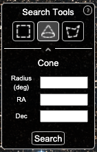
To search by cone (circle on the sky), click the cone icon and press and drag the cursor in the sky. A green circle will appear to indicate the search area and shows the size of the radius in degrees. Release the cursor and the circle will appear highlighted in the sky and values for the radius, RA and Dec will appear in the search tools window. These values can be changed in the window. The count numbers for images, catalogues, spectra and light curves updates. Search for any data now using the top left icons and the results will only contain data that fall within the specified radius (note all data with footprints falling partially within the region will also be retrieved).
To search in a box or rectangular region of the sky, click the square icon and press and drag the cursor. A green box will appear to indicate the search area. Release the cursor and the box will appear highlighted in the sky and values for the BOX in an STC-S string format appear in the search tools window. These values can be changed in the window and follow the format: BOX ICRS RA(1) DEC(1) RA(2) DEC(2) RA(3) DEC(3) RA(4) DEC(4). See the search tools window more information for examples.
To search in an arbitrary shape on the sky, select the polygon search icon. Click anywhere in the sky, move the cursor and click again at least 3 more times, selecting the region. To complete the polygon, either double click or press the first point. The polygon will appear highlighted in the sky and values for the POLYGON in an STC-S string format appear in the search tools window. These values can be changed in the window and follow the format: POLYGON ICRS RA(1) DEC(1).... RA(n) DEC(n). See the search tools window more information for examples.
SKIES MENU
The top left of the interface shows the coordinates of the cursor, the coordinate system, Equatorial (J2000) or Galactic, the field of view (FoV), the sky that is currently being displayed, and below this, a line of buttons. The first to the left is the skies icon:

Clicking on the icon brings up the Skies menu. The skies are ordered into wavelength regions, from Gamma-ray to Radio, and an Others section at the bottom which currently holds physical models. Select a sky by choosing the wavelength region in the first panel, and browse the skies in the second panel. Details on each sky can be found by clicking the i icon. For further details and a list of all the available skies, go to the skies (HiPS) information page.
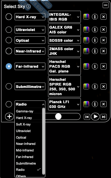
The colour of the skies can be modified with the colour map options 'Native', 'EOSB', 'Planck', 'Rainbow', 'Greyscale' and 'Cubehelix'.

A sky can be added to the stack by selecting the + button:

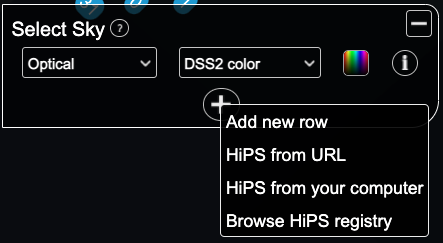
Since version 3.9, it is possible to add a HiPS generated by the ESASky team (Add new row), load it from an URL (HiPS from URL), from your local repository (HiPS from your computer) or browse a HiPS registry for globally available HiPS (Browse HiPS registry):
Click on the video style buttons to play through the skies in the stack, skip forward, backwards or stop.

Since version 3.2, you can also move between skies using the slider:

DATA PANEL (Imaging, Catalogue and Spectra Search)
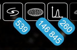
To search for imaging, catalogues or spectral data (and to open the data panel) click on the respective imaging, catalogue and spectra icons in the left menu. The numbers correspond to the number of imaging data, catalogue sources and spectral data that are available for the region of the sky displayed in the browser (not just for the searched target):
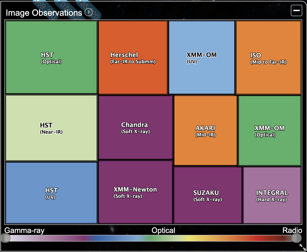
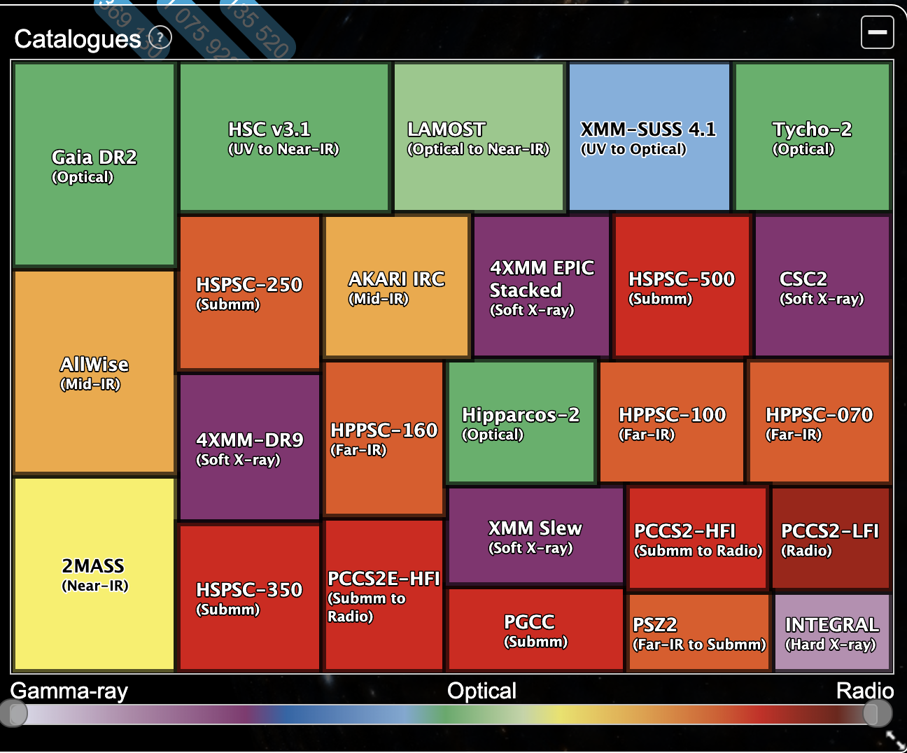
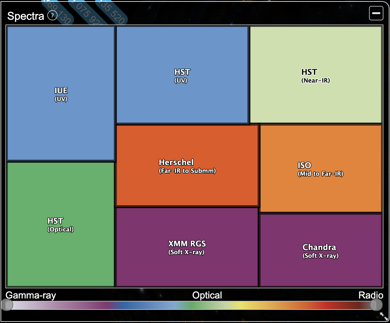
Clicking on one of the menus brings up a treemap which shows the imaging catalogues or spectral data for each mission. The size of the boxes within the treemap are proportional to the number of observations available, with the largest box always appearing in the top left. The wavelength regions are included with the mission names and the missions, the majority of the time, are colour coded by wavelength, with Gamma, X-ray & UV appearing blue or purple; Optical appearing green; and IR to Radio appearing orange and red. As said above, these results are for the entire area being displayed, not just for the source. The results being shown are the highest level science observations only.
 |
 |
 |
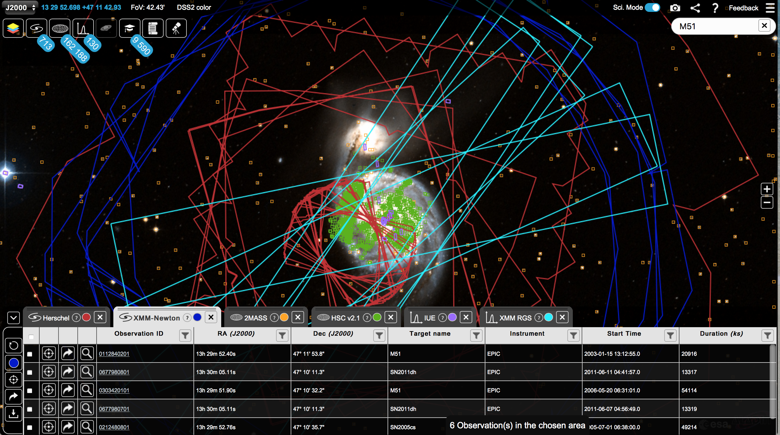
The treemaps are interactive, use the slider at the bottom to select a wavelength range, the available missions in the given range are then shown. Click on each mission to query the archives and load either the images, catalogues or spectra for the region, depending on the treemap selected. A results table appears with the observation or catalogue details and the footprints of the observations or catalogue sources are drawn on the sky. Clicking on an observation or catalogue source will highlight the corresponding observation footprint or source in the sky, and vice versa:
The colours and thickness of the contour lines of imaging and spectroscopic footprints can be changed by clicking on the "Customise" button to the left of the data table (the colour of the circle will match that of the footprints):

Also the shape and colour of the symbols showing the positions of catalogue sources can be modified using this functionality.
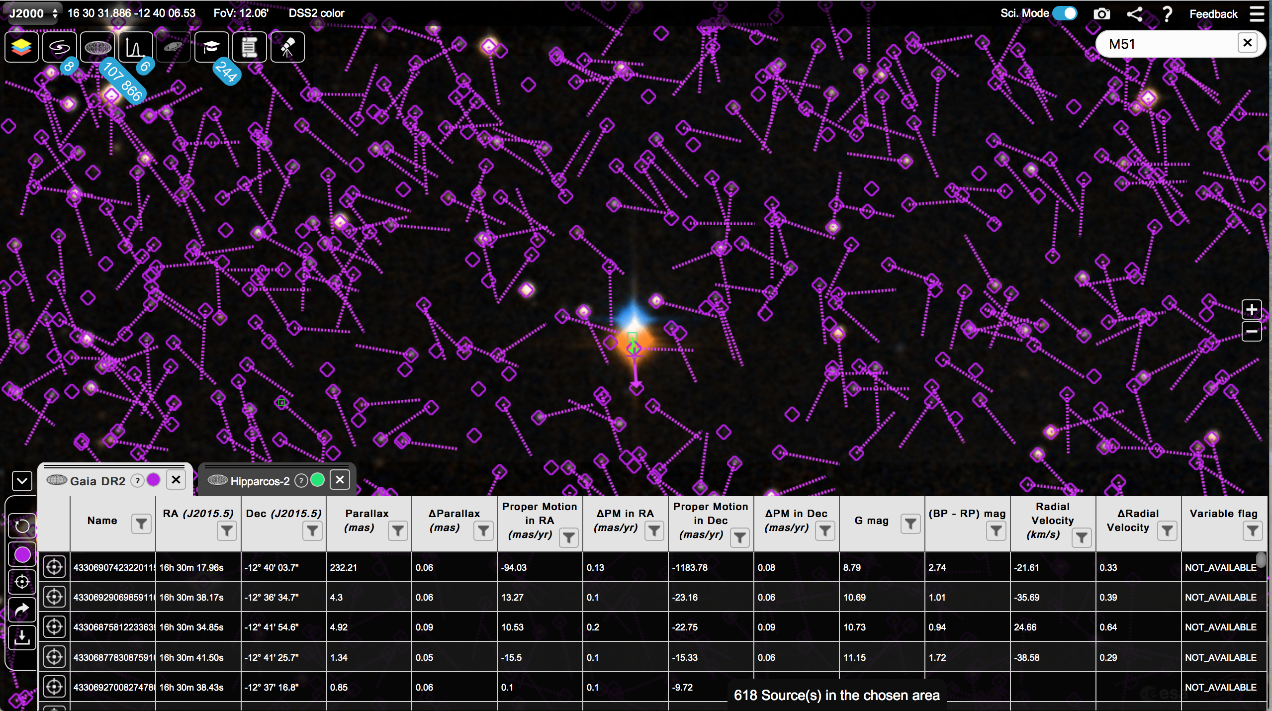
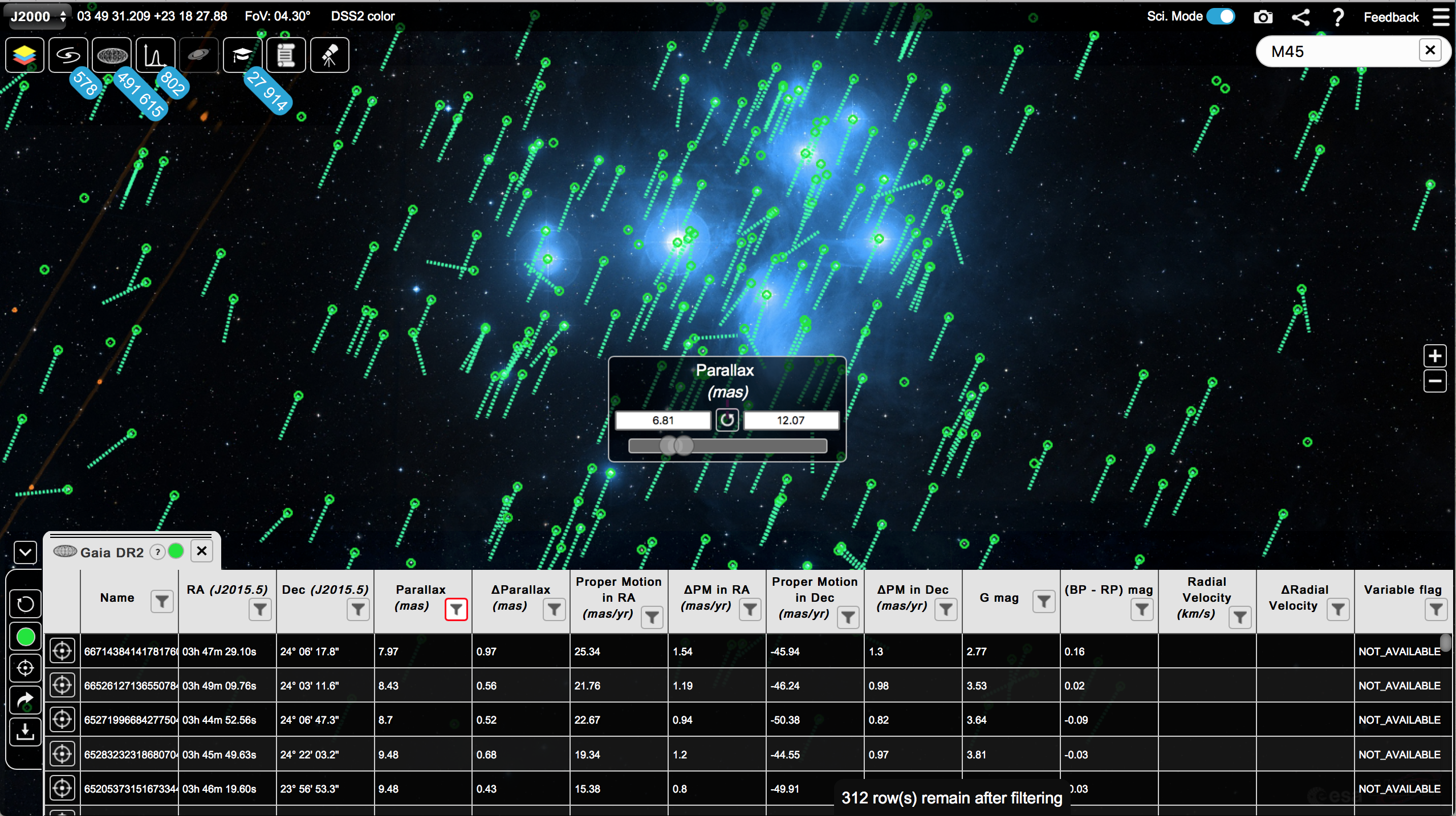
If a catalogue contains proper motion information, ESASky displays not only the position of the sources as defined in the catalogue, but also the direction of motion. In a large field of view, this is shown with a dotted line; the length of the line is proportional to the total proper motion value, but it does not represent the precise movement. The colour and length of this line can be customised by the user.
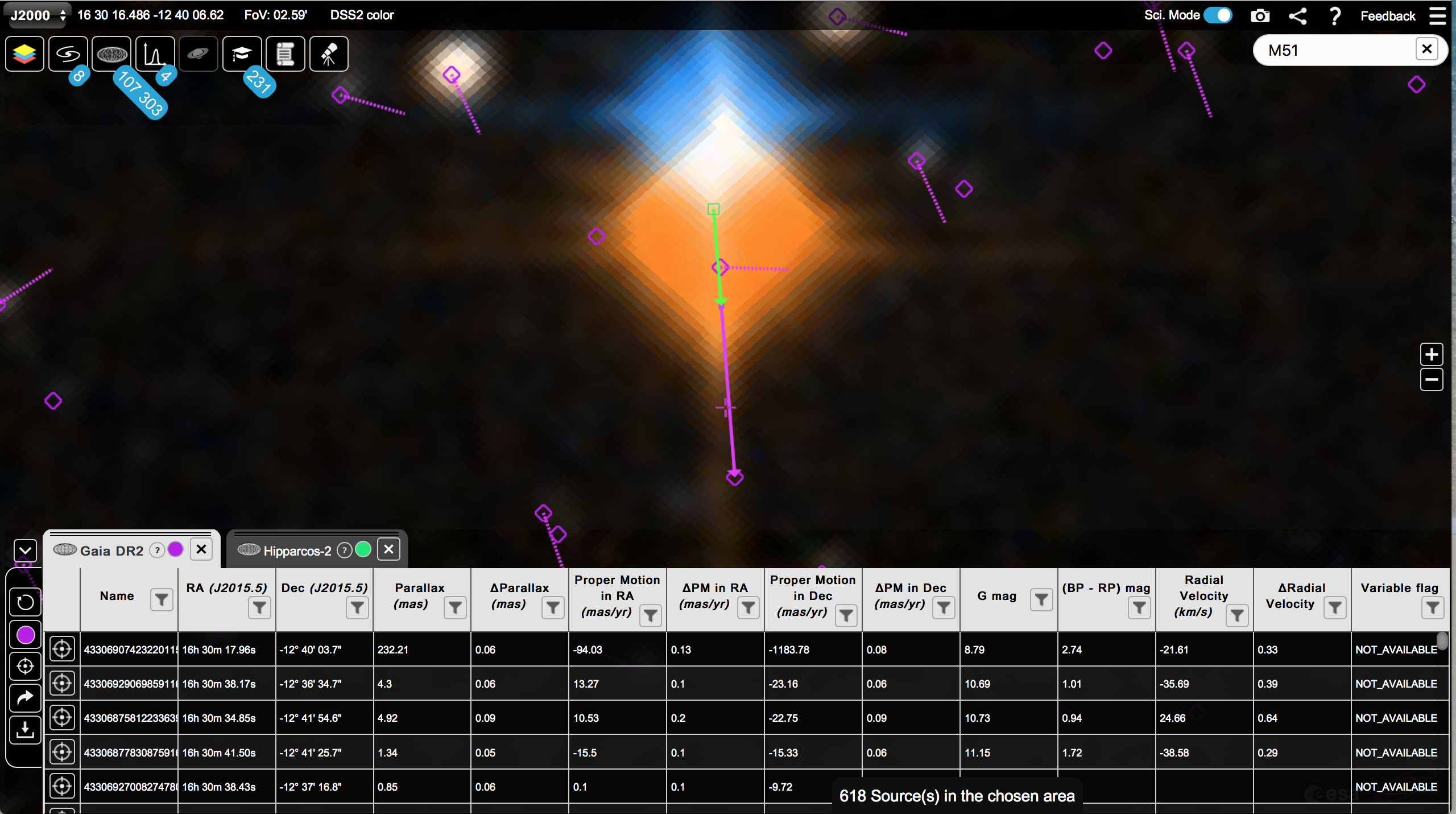
Once you zoom in, the dotted line is replaced by an arrow showing the motion of the source between the catalogue's reference epoch (indicated in the labels of the RA and Dec columns in the data table) and J2000. For example, in the case of Hipparcos, the arrow starts in J1991.25 and ends in J2000; while in the case of Gaia DR3, the arrow starts in J2000 and ends in J2016.0. In both cases, the square represents the original catalogue position (J1991.25 for Hipparcos and J2016.0 for Gaia). Clicking on the Customise button, it is possible to change the colour of the arrow (but not its length), and to subtract the mean or the median of the proper motions of all the stars in the field of view.
Columns in a table can be sorted by clicking on the column's header, and filtered using the funnel button:
It is possible to filter on strings, numerical values and dates. With strings, users can concatenate more than one condition in the same filter with the "|" symbol, which represents the logical OR. With numbers, it is also possible to set a range of numerical values, either with the slider or manually entering the upper and lower values. When a column has been filtered, the funnel button is highlighted in red, and the number of rows displayed after filtering is displayed at the bottom of the screen.
Clicking on the search icon of each row will retrieve the observation postcard directly from the corresponding mission archive:

Clicking on the SAMP button will send the corresponding image to a SAMP (Simple Application Messaging Protocol) enabled application (e.g. DS9, Aladin):

Finally, within the results table, each observation or source can be centred on by clicking the 'Centre on observation' or 'Centre on source' button:

To download the observations, tick the left boxes (or the top left box to select all observations), click the 'Download' button (located to the left of the data panel) and choose 'Download data products'.

The Download menu also provides the option to save the results table in CSV or VOTable format. The results table can also be sent via SAMP to a SAMP enabled application (e.g. TOPCAT) by clicking the SAMP button in the left menu  . The top icon in the left menu of the data panel is to refresh the mission/tab data
  . For example, if you zoom out or pan to a different part of the sky, you can reload the mission/catalogue data for the displayed region by clicking the refresh icon. Also, if you have panned to another region or performed another search, you can go back to the tab's original search field by clicking on the 'recentre' icon in the left menu:
  .
.
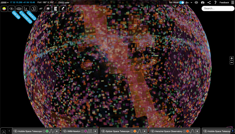
To visualise the sky coverage of all the available ESA missions, zoom out to a distance where the treemap is showing that thousands of observations are available (or zoom out to view half the sky) and then click on one of the missions. A message will appear showing the total amount of objects (observations or sources) in the field of view. If this is below 10 million, then filtering on the data can be performed. The coverage maps are interactive, a pop-up window will appear when a 'tile' in the sky is selected with information on the number of objects available in the tile region per loaded mission. If the objects are below a certain threshold the data can be loaded in the region of the selected tile by clicking on 'load data'. Zooming in will automatically load the footprints and metadata once below a certain number of objects.
The image below shows coverage maps for XMM-Newton X-ray (imaging; purple), Chandra X-ray (imaging; purple), Hubble Space Telescope Near-IR, Optical and UV (imaging; light green, green and light blue respectively), Herschel far-IR to submm (imaging; red) and Spitzer Space Telescop mid to far-IR (orange). As with the footprints, the colours of the coverages are customisable.
SOLAR SYSTEM OBJECTS SEARCH FEATURE
In ESASky, you can search for any planet, satellite or comet observed by HST, Herschel and XMM-Newton (targeted or serendipitous images). Type the name or ID number of the object in the search box and a selection of suggested targets will be given:

Choose the target and the solar system icon will be activated with the number of available imaging observations and the treemap will open:

Select the mission and all available imaging observations will load in the data panel and the footprints will be drawn on the sky. Additionally, the orbit of the solar system object for the entire duration of the mission will be plotted:
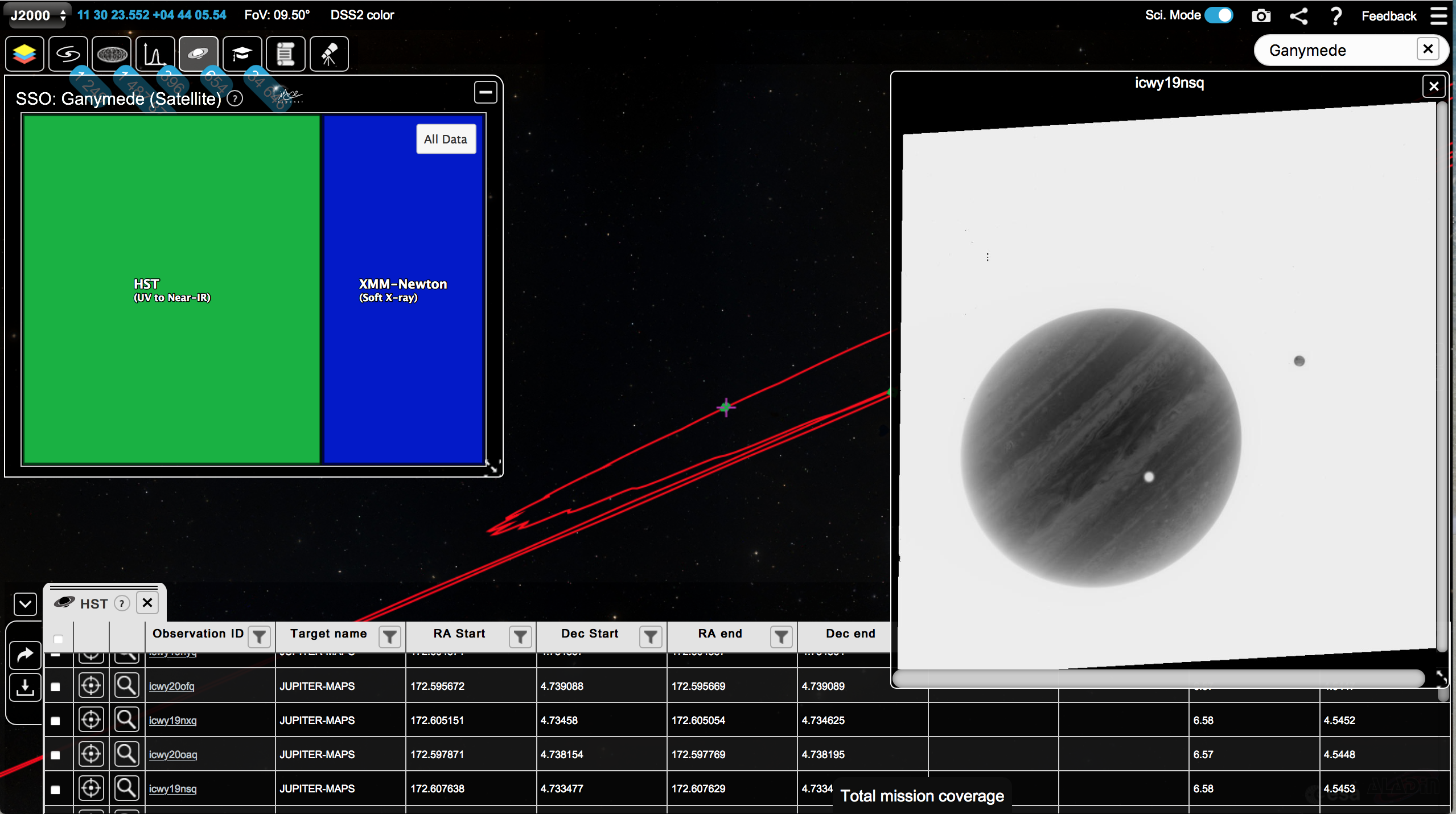
For this feature, the ESASky team has created a pipeline that takes the ephemeris information of each SSO with respect to the position of each spacecraft using software by the IMCCE (Institute of Celestial Mechanica and Ephemeris Calculations, Paris) and performs a crossmatch on the SSO orbits against the entire mission archives to find observations in which the SSO fell within the imaging instrument's field of view during the time the images were being taken.
Imaging observations from other missions will also be added soon.
This short movie shows the SSO feature in action. See Racero, E. et. al. (2022) A&A, 659, 38 for full details.
MULTI-MESSENGER EVENTS
This tool shows public multi-messenger events from gravitational waves and neutrinos, displays their probability footprints on the sky and provides access to the data. Click on the multi-messenger icon to open the window:
![]()
The Gravitational Waves tab displays a list of the gravitational wave events detected by Advanced LIGO and Advanced Virgo from the observing run 3 (O3) and by the LIGO-Virgo-KAGRA collaborations 4th observing run (O4). Click on a gravitational wave event to go to the centre of the associated footprint. A solid line shows the 50% confidence contours and a dashed line the 90% confidence contours. The probability map is also shown. The probability map and contours are extracted from the data available in the GCN webpage, without including the ejected ones. We use the files LALinference when available and Bayestar. For more information visit LIGO collaboration and Virgo collaboration webpages and the Gravitational-Wave Candidate Event Database (GraceDB) webpage. See here for more information on the columns displayed in ESASky.
The Neutrinos tab displays a list of the Neutrino event candidates detected by the IceCube Neutrino Observatory and reported to GCN (Gamma-ray Coordinates Network)/AMON Notices. Gold, Bronze and Cascade candidate events are displayed and the list is automatically updated when new events are reported in the GCN Notices. Gold and Bronze events are single-neutrino events in the IceCube detector with a neutrino energy between sub-PeV to 1 PeV. Gold events are on average ~50% likely to be of astrophysical origin and Bronze events are on average ∼30% likely to be of astrophysical origin. Cascade events are triggers from high energy neutrinos.
When the Neutrino tab is selected, all IceCube Neutrino candidate events are listed and the footprints are displayed on the sky. The footprints are the location uncertainty (a radius, statistical plus systematic, 90% containment. The 'Src Error' column, or the 'Error90' column in the GCN/AMON). Click on the 'Go to' button to centre on each event and the 'Event Page' to view the GCN/AMON notice for each event. For more information visit the IceCube Neutrino Observatory and the GCN/AMON webpages. See here for more information on the columns displayed in ESASky.
SCIENTIFIC PUBLICATIONS SEARCH FEATURE
In ESASky, you can now search for SIMBAD sources with scientific publications from the Smithsonian/NASA Astrophysics Data System (ADS). The publications tool has it's own button (an academic hat):

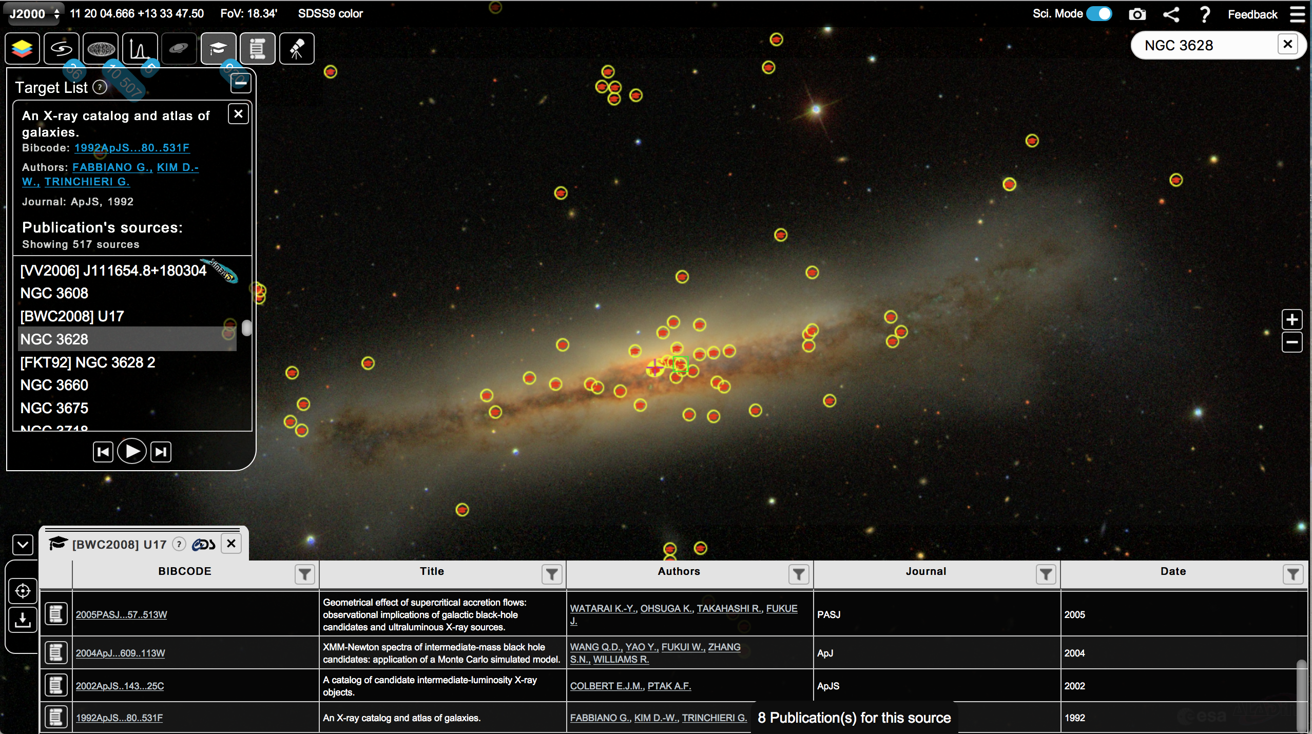
Once the icon is selected, the sources containing publications are shown (with a yellow and red icon) in the displayed field of view. The display can be updated automatically when changing the field-of-view by selecting the "Update on move" option. It can also be updated manually with the "Refresh" button.
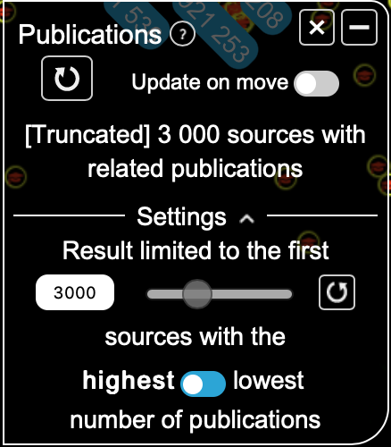
If the number of sources is very high, the list will be truncated (by default) to the 3000 sources with highest number of publications. This can be customised by clicking on "Settings" and playing with the available options. The "Refresh" button next to the slider will reset to the default values.
Clicking on each source loads a table with the publications for that object, including a link to the paper in ADS, the title, authors, journal and date. The first column contains a button to load the sources from each individual paper (obtained from SIMBAD):

The sources are loaded into a target list and can be browsed through, object by object, to visualise them on the sky.
To deactivate the publications tool, click again on the publications icon. Please note that we currently have a limit of 3000 on the number of papers per source that can be displayed and sorted in the results table:
It is also possible to search for publications by author or bibcode, simply entering it in the search field (go here to see the formats). If an author's name is entered, a table will open with the author's publications that are linked to sources in SIMBAD, and the list of sources will be uploaded. Entering a bibcode, the list of related sources in SIMBAD will be uploaded.
EXTERNAL Data Centre (TAP) SEARCH
In ESASky, it is possible to query data from external data centres via their Table Access Protocol (TAP) services compliant with Virtual Observatory (VO) standards. Since version 5.0 of ESASky, this functionality has been expanded to include data from any external TAP of the user's choice. The dashboard functionality of the tool includes the data provided by the European Southern Observatory (ESO), the Canadian Astronomy Data Centre (CADC), the Mikulski Archive for Space Telescopes (MAST), the High Energy Astrophysics Science Archive Research Center (HEASARC) and the Netherlands Institute for Radio Astronomy (ASTRON) in their TAP servers, including images, spectra, data cubes and time series data. Any other TAP with an ObsCore table can also be added to the dashboard (see below for details).
Additionally, access to the VizieR Astronomical Catalogue Service from the Strasbourg Astronomical Data Center (CDS) and access to ESA TAPs are conveniently provided from their own tabs, and the TAP Registry tab allows users to search and load metadata from any TAP registered in the VO. Any TAP tables can now be loaded into ESASky (with a limit of 10000 rows). The column metadata for each table can also be loaded and tables can be queried using the Astronomical Data Querying Language (ADQL), again with a limit of returning 10000 rows. The main reason this limit is applied is to not overload the browser's memory and affect the performance of the tool. Users can toggle the field of view (FoV) button on or off, to obtain data within the FoV displayed in ESASky, or data from the whole sky, including entire catalogues. Continue reading below to learn how to use these new functionalities!
Please note that these data, contrary to those offered via the images, spectra and catalogues functionalities in ESASky, have not been curated by the ESASky team.
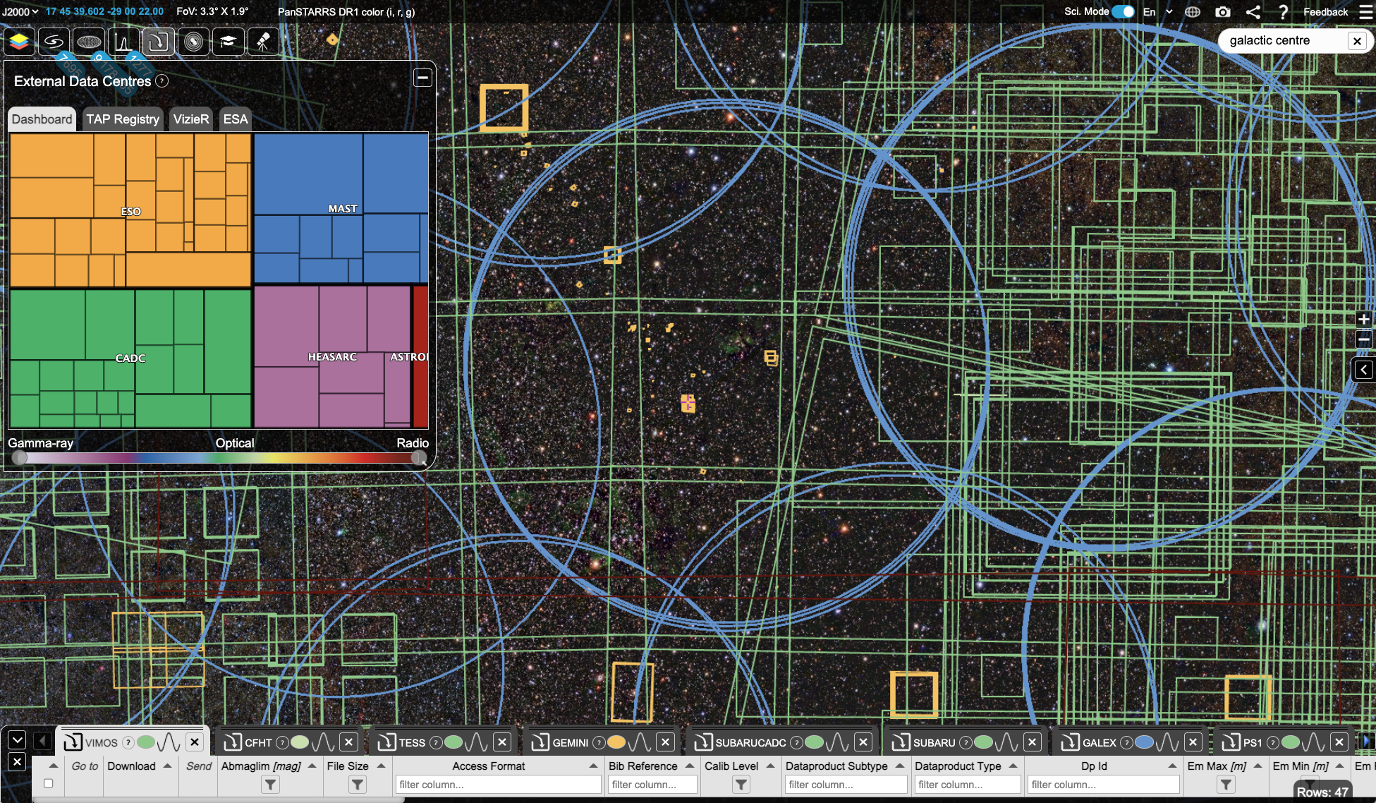
To use this functionality, click on the External Data Centre button:

This will open a treemap showing the servers with data available in the visualised region. Clicking on any server, the treemap will display the types of data products available:
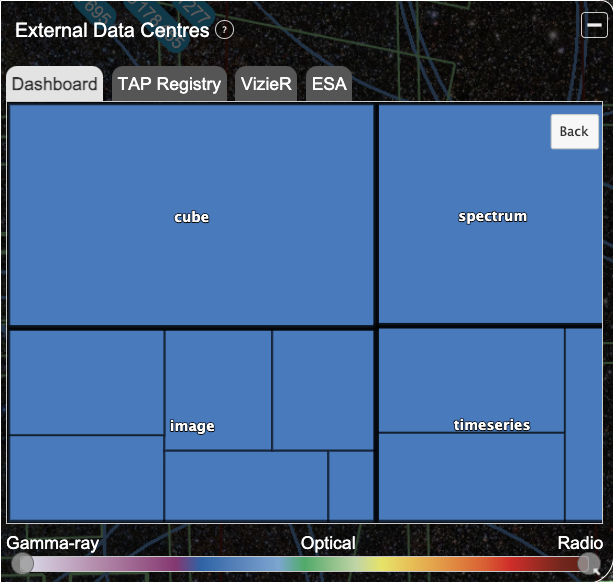
Clicking on any data product will display the data collections available:
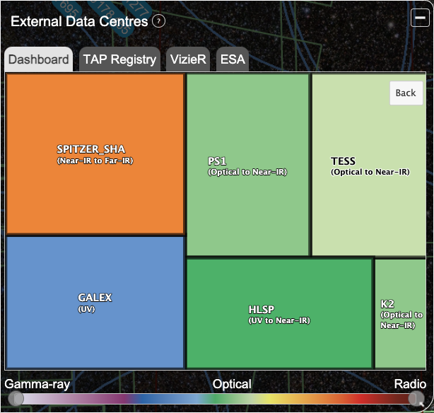
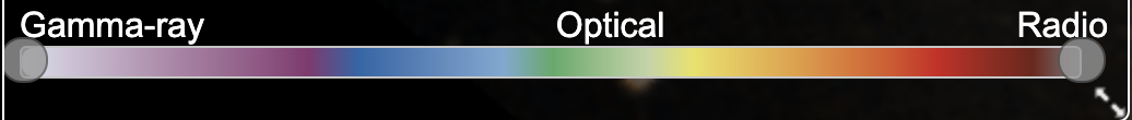
It is possible to change back to the previous treemap level with the "Back" button or to filter the missions/telescopes by wavelength using the slider at the bottom of the treemap:
Clicking on a collection, the corresponding metadata table will open in the data panel, and the footprints will be displayed on the sky. The table can be browsed, filtered, resized and downloaded in the usual way. To download a particular data product, click on the corresponding download button in the 'Access Url' or 'Download' column:
A window will pop-up with information on the files available in the server for this product, which can be downloaded by clicking on the corresponding link.
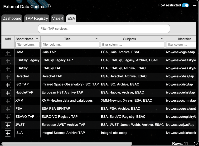
Clicking on the 'TAP Registry' tab will display all TAPs available in the VO TAP Registry:
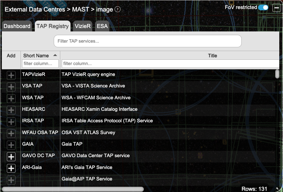
TAP services can be searched for in the 'Filter TAP services' field at the top of the window. And all columns displayed can also be filtered.
If a TAP has an ObsCore table, the button in the first column, titled 'Add', will appear highlighted. This ObsCore table can be added to the main dashboard by selecting the + button:

If data from the selected TAP ObsCore table is availalbe in the field of view, then the service will appear in the dashboard and footprints and metadata from the ObsCore table can be loaded in ESASky in the same manner as the default Data Centres:
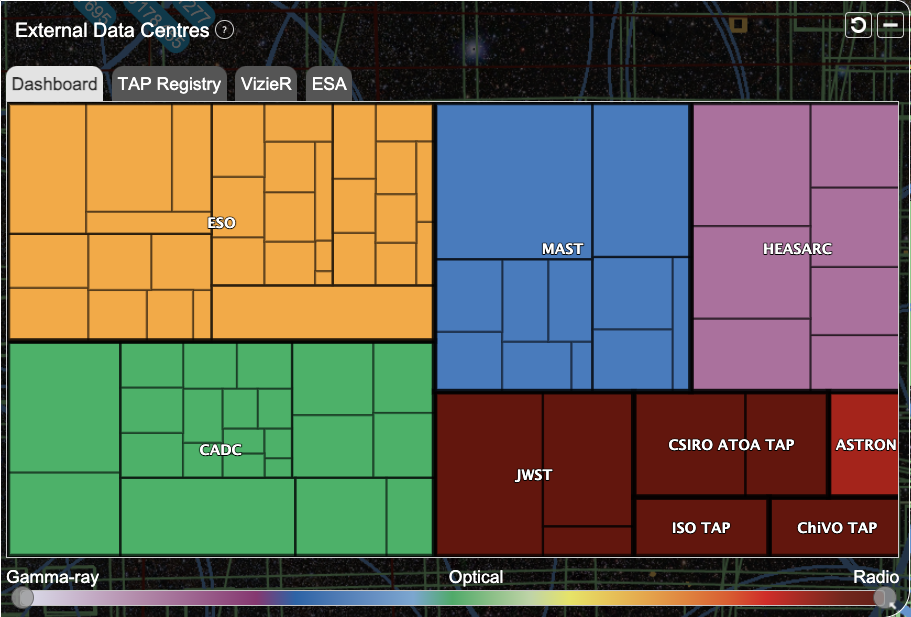
To remove any added services, select the reset button in the top right of the window and only the default services from ESO, CADC, MAST, HEASARC and ASTRON will again be shown:

To load any table from any TAP service, select the TAP Registry tab and click on the name or title of the service you want to explore. The folders of each TAP are shown in a tree structure and can be opened by clicking on the row. Tables can be searched for via the 'Filter TAP tables' field or by using the column filters:
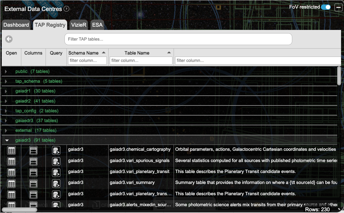
Clicking on the table button will load the table data into the data panel:

Toggle the field of view (FoV) button, called 'FoV restricted' on or off, to obtain data within the FoV displayed in ESASky, or to obtain data from the whole sky, including entire catalogues (limited to 10000 rows):

If ESASky can not find any columns defining the coordinates or region, a window will pop up asking if you wish to assign the columns manually, or instead load the entire table:
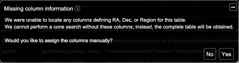
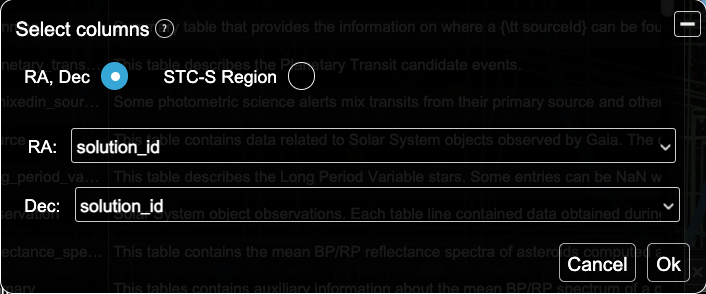
Selecting yes will open another window where you can manually select the RA, DEC or STC-S region columns:
Clicking on the column button will load the table column metadata into the data panel:

Click on the ADQL button to query the selected TAP with an Astronomical Data Querying Language (ADQL) query:

ADQL is based on SQL (Structured Query Language), which is a language to retrieve information from tables stored in a database. When the ADQL button is selected, a window opens and any custom ADQL query can be added to the main field:
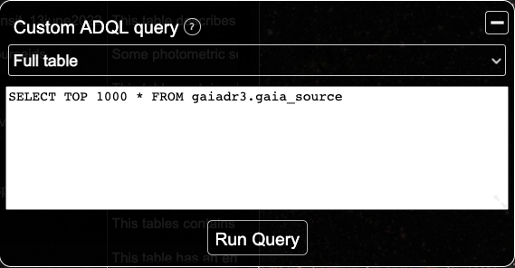
Example ADQL queries can also be selected in the drop down menu, such as: 'Full table' (a 'SELECT TOP' query), 'Columns in table' and 'Count rows'. The ESA Gaia Archive ADQL help section provides a good list of ADQL tutorials and resources for newcomers learning ADQL. Tip: hovering over the tabs in the data panel for each query using the External Data Centres feature will show the ADQL used for that query.
The VizieR tab in the External Data Centres window provides convenient access to the VizieR TAP (called TAPVizieR), which gives access to all tables published in the VizieR Catalogue Service by the Strasbourg Astronomical Data Center (CDS). Clicking on the VizieR tab will open the list of folders in the TAP, in a tree structure and clicking on the row will open the folder. All folders and tables in VizieR are loaded (regardless if the FoV restricted button is toggled on). Since there are almost 53,000 tables (and counting!) in VizieR, we recommend using the filter fields to find your catalogues of choice:

Loading table data, column metadata and querying with ADQL are all identical to the TAP Registry tab, e.g. using the 'Open table' button, 'Show column metadata' button and ADQL button respectively. A message is given if a table is loaded but does not contain data in the field of view. Untoggle the 'FoV restricted' button to load the entire table (restricted to 10000 rows).
The ESA tab in the External Data Centres window provides convient access to all TAPs provided by ESA. Functionalities in this tab are identical to those in the TAP Registry tab:
See also the following video: Announcing ESASky version 5.0: Access to VizieR and more Data Centres!
TARGET LISTS
The 'upload target list' icon can be found in the search field, and in explorer mode it is also one of the top left icons:

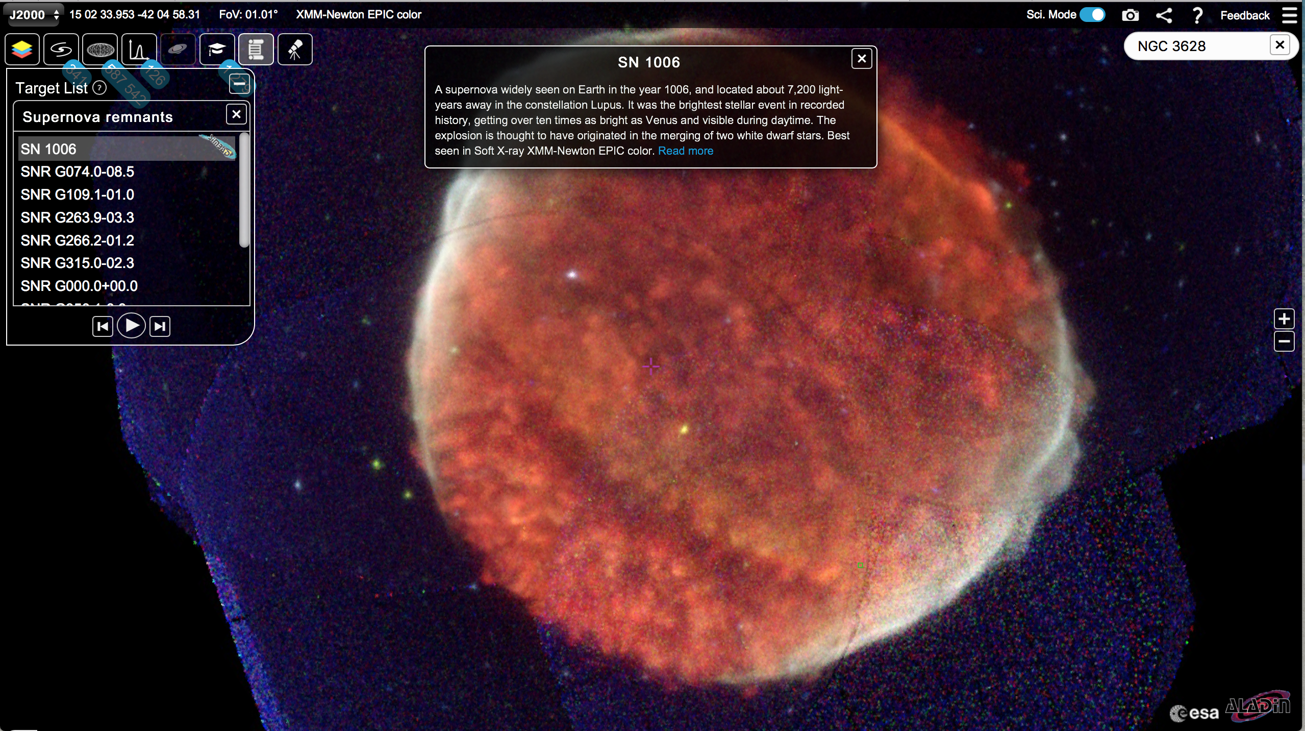
You can choose to either select a predefined target list, grouped by type of object:
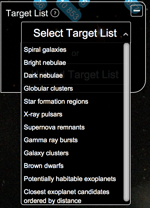
or you can upload you own text file containing your list of targets, either names resolved by SIMBAD or a list of coordinates. While the list is loading, the message 'Resolving target list...' appears at the top of the interface, then once loaded, the target list appears on the left. Click on a target to view it in the sky. If an object has not been resolved by SIMBAD it will be crossed out. Below the target list are some video style buttons, press play to play through the list of targets, the target being displayed will be highlighted in dark grey in the list. Text and comments can also be added to a target list and the text is displayed in ESASky in a separate window. See here for the format needed to display text and some example files.
OBSERVATIONS PLANNING TOOL
The observations planning tool icon lies in the top left menu, next to the Multi-Messenger icon:

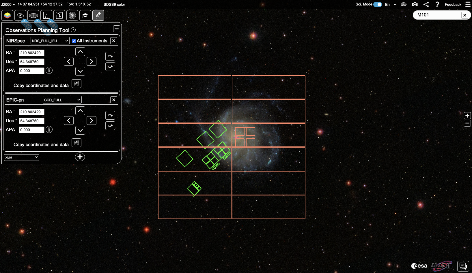
This tool projects onto the sky the footprints of astronomical instruments, at any chosen position and orientation, and has been developed to aid professional astronomers when they are defining their future observation proposals for a particular space mission or ground-based telescope. Currently the tool works for all the James Webb Space Telescope (JWST) instruments (including being able to project the full focal plane of the JWST), and for the XMM-Newton EPIC-pn camera.
IMPORTANT: This functionality is not intended to replace the JWST ATP tool, but just to provide a quick-look aid for astronomers planning JWST observations that require overlapping with existing observations by other missions available in ESASky, or who want to make sure that their instrument or parallel pointings are covering/avoiding particular features or objects in their target regions. The coordinates and positional angles of the pointings defined using this functionality have to be checked and refined in the APT, which is the official tool for preparing JWST observations. For information and installation of the APT, go to this STSci webpage; for details on the different JWST instruments, click here.
ESASky uses the Aladin version of the EPIC-pn footprint template, see here for more information (in the proposal submission procedure and tools section). ESASky uses the latest version of the JWST SIAF (version number shown in the bottom of the planning tool window from ESASky v3.5 onwards). The SIAF is a reference file used in operations that contains the official information on all apertures (e.g., NIRCam Apertures) and internal instrument coordinates. The JWST Project Reference Database serves as the repository for operations reference files like the SIAF, its version number is a unique identifier of the reference files that it bundles. APT prompts the PRD version number used for observations preparation, see here for further information.
Clicking on the icon opens the observations planning window, and clicking on the plus '+' opens the instruments menu:
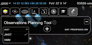

When an instrument is selected, the corresponding footprint aperture is displayed in the centre of the field of view. You can change the location and orientation of the aperture with the arrows, or by typing into the fields. The rotation (APA, or aperture position angle) is the angle specific to the instrument field of view (in degrees). For the JWST instruments, this is regardless of its offset angle relative to the Observatory V3 axis. This parameter is used to specify the desired orientation of a JWST aperture using the APT special requirements, see here for more information. When the footprint is in the correct position, click on the 'Copy coordinates and data' to get the pointing coordinates and position angle.

By default, each instrument's aperture has a predefined centre. However, it is possible to centre it in a particular aperture by choosing it in the menu:

Clicking on the apertures centres will display a tooltip with the positional information of that centre:

It is possible to display several footprints of the same or different instruments together, and to move and orientate each one of them individually. In case you are planning simultaneous observations with several JWST instruments, there is also the possibility to display and position the full focal plane at once. To do this, check the 'All Instruments' option beside the detector menu. The footprints of all instruments will be displayed with the correct relative positions and distances on the JWST focal plane. Your selected instrument will be shown in red and the other instruments in green.
See also the following video: How to plan future JWST observations
esa/hubble outreach images
ESA/Hubble Outreach images are available in Explorer mode, via the hubble icon: 
Clicking on the icon displays a list of outreach images released by the ESA/Hubble team. Click on a footprint or on a list item and the outreach image is shown overlaid on the sky currently displayed. A text box opens with the description of the image and the link to its location on the ESA/Hubble website. You can play with the opacity by moving the Image Opacity bar to the left and to the right. See here for more details about the feature.
IMPORTANT: These images are created for outreach purposes and they are not intended for scientific use.
ESA/WEBB outreach images
ESA/Webb Outreach images are available in Explorer mode, via the hubble icon: 
Clicking on the icon displays a list of outreach images released by the ESA/Webb team. Click on a footprint or on a list item and the outreach image is shown overlaid on the sky currently displayed. A text box opens with the description of the image and the link to its location on the ESA/Webb website. You can play with the opacity by moving the Image Opacity bar to the left and to the right. The ESA/Webb, ESA/Hubble and Euclid Outreach Images features can be opened together, allowing users to switch between and compare the awe-inspiring outreach images from Webb, Hubble and Euclid. See here for more details about the feature.

Euclid outreach images
Euclid Outreach images are available in Explorer mode, via the Euclid icon:
Clicking on the icon displays a list of outreach images released by the ESA Euclid mission. Click on a footprint or on a list item and the outreach image is shown overlaid on the sky currently displayed. A text box opens with the description of the image and the link to its location on the Euclid section of the ESA website. You can play with the opacity by moving the Image Opacity bar to the left and to the right. The ESA/Webb, ESA/Hubble and Euclid Outreach Images features can be opened together, allowing users to switch between and compare the awe-inspiring outreach images from Webb, Hubble and Euclid.

SNAPSHOTS
In the top menu, on the right, lies the snapshot icon:

Click on this icon to take a screenshot of your displayed ESASky screen (including any observational footprints and catalogues also displayed on the screen) and save it as a png file. A number of your png files can then, for example, be combined into an animated gif (note: locally on your computer, not currently with ESASky). The following animated gif shows M31 in Soft X-Rays (XMM-Newton EPIC color), Optical (DSS2 color), Mid-infrared (AllWISE color), Far-infrared (Herschel PACS RGB 70+160), Submillimetre (Herschel SPIRE RGB 250+350+500) and Radio (NVSS intensity maps), with the Gaia DR1 TGAS (orange squares) and XMM-slew (light blue squares) catalogue sources:
SELECTION TOOL
New to version 3.9, when opening an image/catalogue/spectra the selection tool is automatically displayed in the middle right part of the screen. This tool allows the selection of sources/footprints within a selected area.

There are three shapes available: square, circle and polygon. For the square and circle, to select sources or footprints in the sky, press and drag from top-left to bottom-right. A green box or circle will appear to indicate a selection area. Once you are satisfied with an area, release the pointer and every source under the area will be selected. To deselect, do the same operation, but press and drag from bottom-right to top-left instead, creating a red deselection area. The polygon tool allows the selection of sources/footprints within an area of an arbitrary shape. Each touch or click adds one point to the polygon. Finish the polygon by either double clicking or pressing the first point. It is possible to enter selection mode by holding the Shift key. You will stay in selection mode as long as the shift key is pressed, allowing you to do multiple subsequent selections.

EXPLORE RANDOM TARGETS FEATURE

Roll the dice and take a tour through the cosmos! In explorer mode, click on our explore random target icon (dice icon) and enjoy discovering and reading about different types of astronomical objects in the sky.
Found your own amazing sources in ESASky? Tell us here and we'll add them to the list!
BOOKMARK / Sharing

By clicking on the bookmark / sharing icon on the top bar, the URL of ESASky is copied onto your computer's clipboard. This URL contains information on the target/coordinates, the background sky, the field of view, and coordinates frame. When copied into a new tab, ESASky loads on exactly the same coordinates, with the same background sky, field of view and coordinates frame. This link can then be shared, for example, via social media or with collaborators, to share interesting objects or regions of the sky. Below are some examples of the bookmarks feature:
- Load ESASky with the HST ACS sky: http://sky.esa.int/?action=goto&hips=HST ACS
- Load ESASky on M101 with the default sky: http://sky.esa.int/?action=goto&target=m101
- Load ESASky on M101 with the Herschel PACS RGB sky, a field of view of 29.77 arcminutes and the Galactic coordinate frame: http://sky.esa.int/?action=goto&target=m101&hips=Herschel%20PACS%20RGB%2070,%20160%20micron&fov=0.4962412691936891&cooframe=GAL
- Load ESASky on coordinates RA = 225.7308 and DEC = -41.9379 (in decimal degrees), with the XMM-Newton EPIC color sky, a field of view of 1.5 degrees and the equatorial coordinate frame: http://sky.esa.int/?action=goto&target=225.7308%20-41.9379&hips=XMM-Newton%20EPIC%20color&fov=1.5&cooframe=J2000
- Load ESASky in the Galactic coordinate frame, on coordinates LON = 353.7716 and LAT = 10.9964 (in decimal degrees), with the Planck HFI 217 GHz sky, and a field of view of 81.8 degrees: http://sky.esa.int/?action=goto&target=353.7716 10.9664&hips=Planck HFI 217 GHz&fov=89.2&cooframe=GALACTIC
The sky (HiPS) name must be the one appearing in the ESASky skies menu. The target name will be resolved by SIMBAD.
AdditionaL Information and HELP MENUs

There are two buttons on the top bar for help and additional information: The first, a question mark, links directly to the 'How to' page. The second, "Feedback", gives access to the ESASky Userecho community. The last button on the right corner brings up a menu with other help and information resources, as well as a link to the World Wide Telescope.
SAVE AN ESASky SESSION
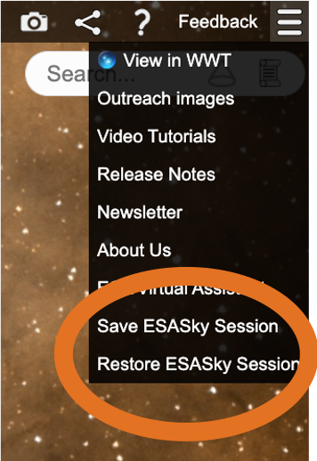
New to version 4.1, you can now save an ESASky session and restore it at a later time or send it to collaborators. Select 'Save ESASky Session' in the hamburger menu in the top right. A json file is then downloaded to your computer. Reload ESASky, for example at a later date, select 'Restore ESASky Session' and select the saved json file. The features that can be saved are: the target/coordinates; the field of view; the coordinate frame and grid; the background skies (HiPS); the active search region (cone, box or polygon); all loaded and filtered data (images, catalogues, spectra, light curves, external data centres) including colour and shape changes; data loaded from the Multi-Messenger window, loaded publications; planning tool options; and the ESA/Hubble outreach images. Note, this feature is currently only available in Science mode and in English.
User Area
New to version 6.0, user areas are now available in ESASky! By creating a user account (ESA cosmos LDAP) and logging into the user area, users can upload their own tables (in CSV or VOTable format), save their ESASky sessions and customise the layout of ESASky. Users have 1 GB quotas (if you need more, please contact us).
Click on the user area icon in the top left of the header ![]() and select 'Login' or 'Register'. You will then go to the ESA Cosmos single sign on service, where you can create your account, and once registered, where you log in. Once logged in, ESASky automatically reloads and asks if you want to continue your (automatically preserved) previous session.
and select 'Login' or 'Register'. You will then go to the ESA Cosmos single sign on service, where you can create your account, and once registered, where you log in. Once logged in, ESASky automatically reloads and asks if you want to continue your (automatically preserved) previous session.
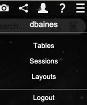
Once logged in, click on the user area icon to access your user profile, tables, sessions and layouts:
User profiles, permissions and quotas can be seen by clicking on the user area icon and then on your user name.
Selecting 'Tables' will open the tables window where tables with CSV or VOTable format can be uploaded by clicking on the blue upload button. Once uploaded, the table will appear as a new row and can be loaded into ESASky by clicking on the open table icon ![]() in the 'Open' column. The table can also be queried and loaded into ESASky with a custom ADQL query
in the 'Open' column. The table can also be queried and loaded into ESASky with a custom ADQL query ![]() .
.
The Sessions feature in ESASky enables users to save the current state of the application, allowing them to revisit their work at a later time. This feature provides users with the ability to capture the current configuration, including the selected datasets, viewing settings, and any customizations made to the interface. By saving this state as a session, users can easily return to where they left off, eliminating the need to recreate their work from scratch. Click on the blue + button to save your current session (which will then appear as a new row in the sessions window).
The Layout feature in ESASky allows you to personalize your viewing experience by arranging and displaying elements within the interface according to your preferences. With this feature, you can easily adjust how different elements are arranged and displayed on the ESASky interface. Whether you prefer certain tools or information to be more prominent or tucked away, you have the flexibility to tailor the layout to suit your needs. Click on the blue + button to save the current layout (which will then appear as a new row in the layout window). Click on the edit button to start your customization. Each ESASky feature is listed, click on the row to either enable or disable the feature (you'll see the feature buttons disappearing and appearing in the interface).