SAS Thread - epatplot - XMM-Newton
How to evaluate and test pile-up in an EPIC source
|
Introduction This thread illustrates how to assess whether an observation is affected by pile-up. Pile-up occurs whenever a X-ray source is too bright for the selected read-out mode, thus in practice is like an overexposure effect.
The effect of pile-up on the spectra is therefore three-fold:
This thread provides a step-by-step description on how to assess pile-up using the pattern distribution and provides one method to minimize its effects and another one to correct for it. Also, this threads explains how to deal with X-ray loading which accompanies pile-up observations. X-ray loading occurs when the count rate is sufficiently high that the offset map, created on-board, is distorted by X-ray photons. The count rate at which this becomes important is discussed in XMM-SOC-CAL-TN-0050. The net effect of X-ray loading is to artificially reduce the energy of events by over-subtracting the dark current in each pixel. The X-ray loading correction is only necessary for EPIC-pn imaging modes. For Timing mode, this is dealt with by SAS automatically, while for MOS, the correction is not necessary. The EPIC-pn offset map has been designed to correct events for optical loading. For this reason it is important NOT to run X-ray loading correction if the source is optically bright. Magnitude limits are given in the Users Handbook. In other words, if the source exceeds the optical and the X-ray limits for the observation mode and transmission filter combination, then the application of the automatic correction for X-ray loading is not possible. Expected Outcome Plot (PS-file) comparing the observed versus the expected pattern distribution within a source extraction region. If both agree, pile-up is not a problem for this source.A response file to be used for correcting the spectra for the flux loss and energy distortion caused by the pile-up of photons. As of SAS v13, this method can only be applied to the EPIC-pn camera in imaging mode, i.e. ExtendedFullFrame, FullFrame, LargeWindow and SmallWindow modes. SAS Tasks to be Used Prerequisites
Useful Links
Last Reviewed: 25 MAY 2023, for SAS v21.0Last Updated: 31 MAY 2018 |
Procedure
- Create EPIC calibrated event list, a corresponding GTI file (see the How to filter EPIC event lists for flaring particle background Thread) and identify the centroid position and extraction radius of your source, for example, using the procedure explained in the MOS or pn spectrum extraction thread.
- Extract a filtered event list, including only photons within the source region, without any filtering in PATTERN or quality FLAG. Assuming that the region has a centroid position (27560,27000) and radius (800) in sky coordinates (X/Y), and that the original event list file name is PN_evt.fits and the GTI file is pn.gti:
evselect table=PN_evt.fits withfilteredset=yes filteredset=pn_filtered.evt \
keepfilteroutput=yes expression="((X,Y) in CIRCLE(27560,27000,800)) \
&& gti(pn.gti,TIME)" - Apply the task epatplot on the filtered event list, pn_filtered.evt, to produce a POSTSCRIPT file displaying the observed versus expected pattern distribution.
epatplot set=pn_filtered.evt plotfile="pn_filtered_pat.ps"
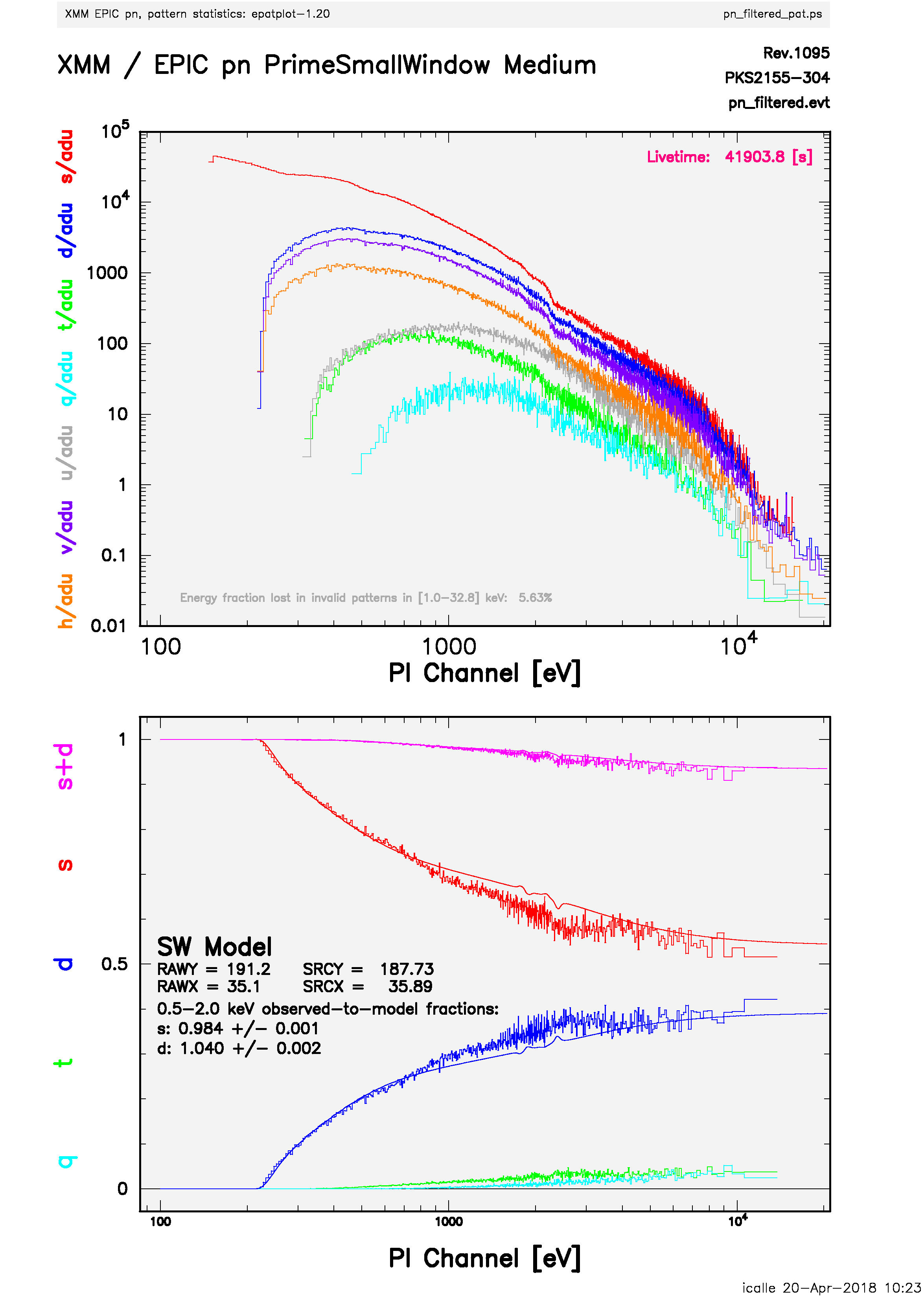
The file pn_filtered_pat.ps contains a plot like the following:

Fig.1: epatplot output file, which in this case indicates the presence of pile-up.
This plot contains two panels:- The upper panel shows a spectrum (distribution of counts as a function of the PI channel: be aware that the counts are not folded with the detector response) for each event pattern class.
- The lower panel shows the expected pattern distribution functions (smooth solid lines) superimposed on the observed ones (histogram). In this panel, also displayed is the observed-to-model fractions for single and double events within a certain energy range.
In all plots, the distributions corresponding to the different pattern classes are recognizable through colors: red for single, blue for double, green for triple, and turquoise for quadruple events.
Your source spectrum will be affected by pile-up if - as in the case shown in Fig.1 - the expected distributions are significantly discrepant from the observed ones. epatplot calculates two diagnostic numbers which may be used to assess the presence of pile-up: In the absence of pile-up, the 0.5 - 2.0 keV (default range) observed-to-model singles and doubles pattern fractions ratios should both be consistent with 1.0 within statistical errors (1 sigma errors are given). If pile-up is present, the singles ratio will be smaller than 1.0 and the doubles ratio will be larger than 1.0. These ratios are both printed to the console and displayed on the plot. They are also added to the header of the input event set as attributes SNGL_OTM and DBLE_OTM (1 sigma errors: ESGL_OTM and EDBL_OTM).
- Below, we provide a way to minimize the effects of pile up and a way to correct for pile up. The pile-up correction method was introduced in SAS v13. While it has been proved to correctly recover flux and spectral shapes for moderately (~a few percent) piled-up sources (see, e.g., the SAS Scientific Validation Reports), its performances for sources affected by a higher level of pile-up have still to be fully assessed. It is then recommended to try both methods and check the consistency of the results. If the results are consistent, pile-up correction should be employed since no photons are discarded by this method.
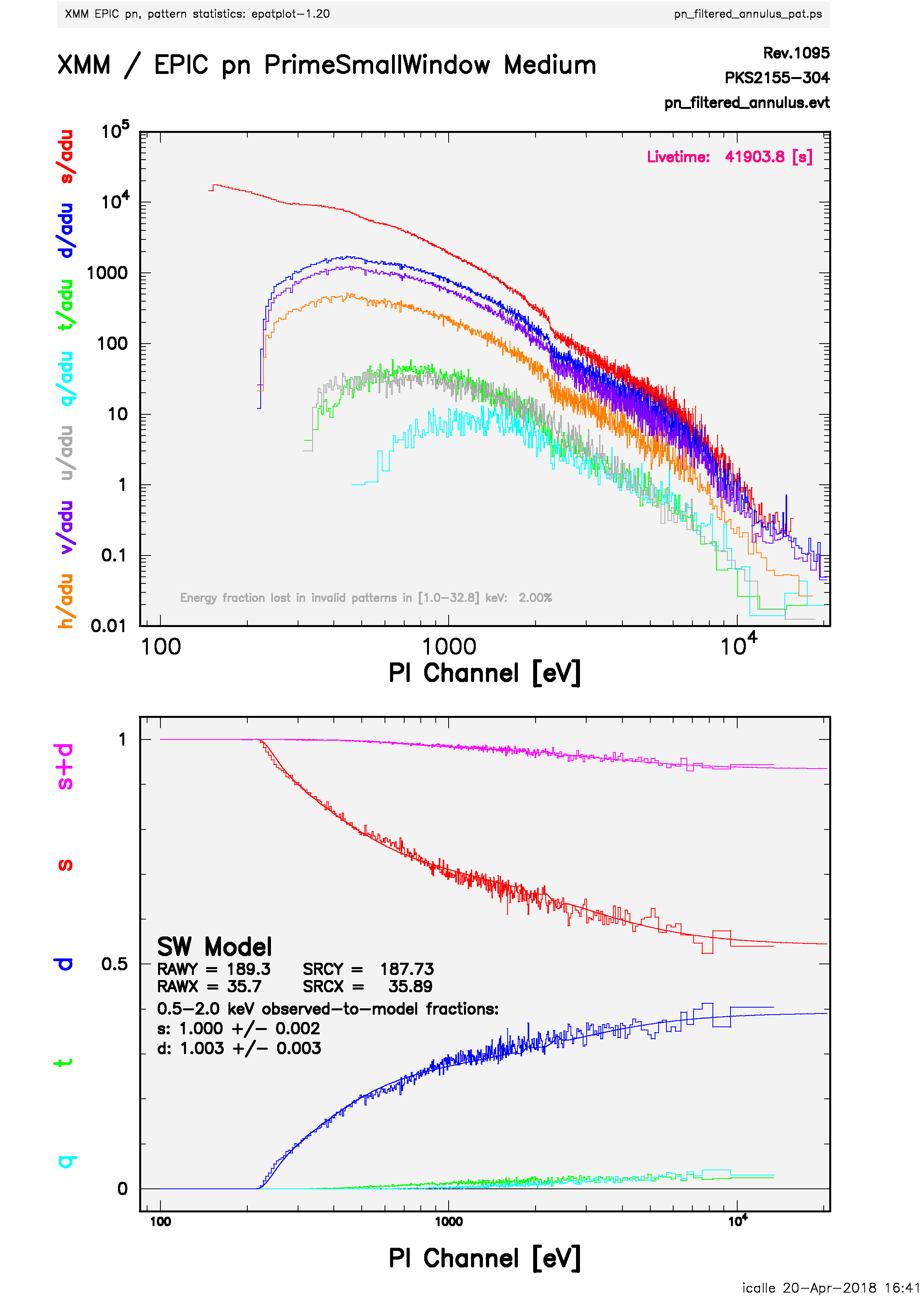
- The way to reduce pile-up in a given data set is to excise the core of the PSF, up to a radius where the pile-up fraction becomes negligible. In order to apply this method, extract filtered event lists of annular regions around the centroid position excising more and more of the core of the PSF until the observed pattern distributions match the expected ones, as presented in Fig.2 below. The following commands excise a radius of 150 from the core of the PSF used in the previous example and creates another pattern plot for this annular region:
evselect table=PN_evt.fits withfilteredset=yes filteredset=pn_filtered_annulus.evt \
keepfilteroutput=yes expression="((X,Y) in ANNULUS(27560,27000,150,800)) \
&& gti(pn.gti,TIME)"epatplot set=pn_filtered_annulus.evt plotfile="pn_filtered_annulus_pat.ps"
The file pn_filtered_annulus_pat.ps contains a plot like the following:

Fig.2: epatplot output file, which in this case indicates a negligible pile-up fraction. - As of SAS v13, rmfgen includes an option to correct for the flux loss and energy distortion caused by the pile-up of photons within a single frame. Currently this is only available for EPIC-pn observations made in an imaging mode (i.e. not Timing or Burst mode). It does this by generating a redistribution matrix that attempts to compensate for the pile-up effects, which are calculated from the frequency and spectrum of the incoming photons. To use this option it is recommended to adopt the following procedure:
- Run the EPIC reduction meta-task epproc to correct for X-ray loading and create an intermediate raw event file by:
epproc pileuptempfile=yes runepxrlcorr=yes
(or epchain keepintermediate=all runepxrlcorr=yes)which produces a calibrated event file, corrected for X-ray loading effects by the routine epxrlcorr, and a raw event file for each CCD with the name *_[CCD#]_PileupEvts.ds (or events[CCD#].dat if epchain has been run).
- Produce a set of spectral files from the X-ray loading corrected event file following the standard procedure. To produce the set of spectral files follow the How to extract PN spectra of a point-like source and associated matrices thread. The set of files generated in this way (spectrum.ds, background_spectrum.ds, myarf.arf and myresp.rmf), will correspond to a spectrum which has been corrected for X-ray loading by the task epxrlcorr but not for pile-up.
- Generate a response file which will include the pile-up correction.
rmfgen spectrumset=spectrum.ds rmfset=myresp_pileupcorr.rmf \
correctforpileup=yes raweventfile=[raw_event_file_for_ccd]the file spectrum.ds corresponds to the spectral file generated in the previous step.
The task rmfgen needs to read a raw event file (raweventfile=[raw_event_file_for_ccd]) to make the pile-up correction. This should contain all the charges which landed on the CCD where the source is centred and was created in step 1. For example, for a source on CCD#4, the file would have a name of the form 2384_0691100201_EPN_S003_04_PileupEvts.ds if produced by epproc and events04.dat if it has been created with epchain.
The pile-up correction technique used is very compute-intensive. The execution times could be of the order of hours for typical observations.
- Once the response file, myresp_pileupcorr.rmf, including pile-up correction is available, we can rebin the spectrum and link all the associated files. In the following example the spectrum is rebinned in order to have at least 25 counts for each background-subtracted spectral channel and not to oversample the intrinsic energy resolution by a factor larger than 3.
specgroup spectrumset=spectrum.ds mincounts=25 oversample=3 \
rmfset=myresp_pileupcorr.rmf arfset=myarf.arf backgndset=background_spectrum.ds \
groupedset=spectrum_grp.fitswhere the files spectrum.ds, background_spectrum.ds and myarf.arf correspond to the spectral files generated in the step 1, and spectrum_grp.fits is the grouped spectrum. The rebinning options shown in the example above, are by no means the only possible binning available, or the recommended one, more binning options are available in the description of the task specgroup.
- Run the EPIC reduction meta-task epproc to correct for X-ray loading and create an intermediate raw event file by:
- We advise to check for pile-up using epatplot even if the count rate of the observation is below the count rate limits of the corresponding mode provided in the UHB.
- The calculated observed-to-model fractions for single and double events within a certain energy range provided in the lower panel of the plot can be incorrect. The important factor is the graphical agreement of the observed (histogram) and expected (solid line) pattern distribution.
- If the statistical quality of the observed pattern distributions (histograms) become too low, the statistical significance used by epatplot can be reduced using the sigma keyword. The following example reduces the default statistical significance of sigma=3 (default) to sigma=2:
epatplot set=pn_filtered_annulus.evt plotfile="pn_filtered_annulus_pat.ps" \
sigma=2
- The energy range of the observed-to-model fraction calculation can be adapted via the keyword pileupnumberenergyrange. The following example switches the default energy range (0.5-2.0 keV) into the energy range used as in Fig.1 and Fig.2:
epatplot set=pn_filtered_annulus.evt plotfile="pn_filtered_annulus_pat.ps" \
pileupnumberenergyrange="1000 5000"
- Excising the core of the PSF on scales too small with respect to the instrumental pixel size (1.1" for the MOS cameras, 4.1" for the PN camera) may introduce systematic inaccuracies in the calculation of the source flux. Simulations show that these systematics are lower than 1% if the radius of the excised core is larger then 5 times the instrumental pixel half-size. For lower sizes these systematics are never larger than 4%. An enhancement of the PSF handling in the SAS is under development to reduce the impact of this effect. In the meantime, users should carefully evaluate the size of the excised core depending on their scientific requirements, and of the source pile-up level. It goes without saying that excising a core, whose size is smaller than the instrumental pixels size, shall be absolutely avoided.
- The way to reduce pile-up in a given data set is to excise the core of the PSF, up to a radius where the pile-up fraction becomes negligible. In order to apply this method, extract filtered event lists of annular regions around the centroid position excising more and more of the core of the PSF until the observed pattern distributions match the expected ones, as presented in Fig.2 below. The following commands excise a radius of 150 from the core of the PSF used in the previous example and creates another pattern plot for this annular region:
