Convolutional Neural network

Convolutional neural network (CNN) is suitable to process image-like data, which can be represented as a matrix with three dimensions – height × width× depth. These type of networks use a special mathematics operation called convolution:

Equation 1

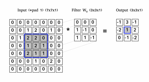
Image 1: Example of convolution. Filter slide on the input with stride two and in every position filter is multiplied with the local regions of the input and then it sums up and produce output.

Like neural network, CNN has the input – input feature maps, weights – sets of filters and output – output feature maps, where all of the mentioned are matrices with three dimensions. Sets of filters contains learnable parameters, which are changed while training. Applying the convolution input feature map are convoluted with set of filters and result is output feature map (Image 1):

Equation 2

An amount of output feature maps is influenced by a number of filters, it is the same as the number of filters. Both height and width are a result of spacial dimension of filters (F), stride and zero-padding. Zero-padding (P) is boarder around input which contains just zeroes. Stride (S) is a step with which is filter moved over the input map. Width (W) or height (H) of output can be calculated as:

Equation 3

Convolution layer can reduce spacial size of the input but more often a pooling layer in employ. Pooling is applied on every feature map separately,preserving the important features in the map. Also, it helps to reduce computational time.

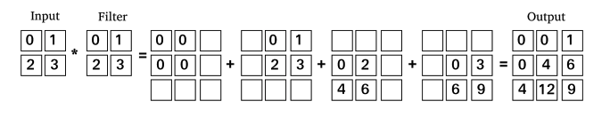
Image 2: Example of transpose convolution operation. This diagram shows one way how to explain this operation, another explanation is Image 3

Another type of layer is a transpose convolution [Dumoulin and Visin, 2016, Odena et al., 2016] sometimes incorrectly named as a deconvolution. The goal of the layer is to increase the spacial size of input layer – it work as up-sample layer (Image 2). Wildly known types of up-sample layers are nearest neighbour and bilinear up-sampling. These algorithms used common interpolations techniques, which estimates values of newly added pixels. Advantage of the transpose convolution are learnable filters which estimate new pixels. Convolution and transpose convolution can be also represented as matrix multiplication. As we can see at Image 3, the convolution is matrix multiplication of filter and the input and in transpose convolution (Image 4), we multiply a transpose filter and the input. In the case of image-to-image translation networks [Chen et al., 2017, Zhang et al., 2019] are usually fully-convolutional neural network [Long et al., 2014] containing convolutional, transpose convolutional (up-sampling) and pooling layer [Goodfellow et al., 2016].

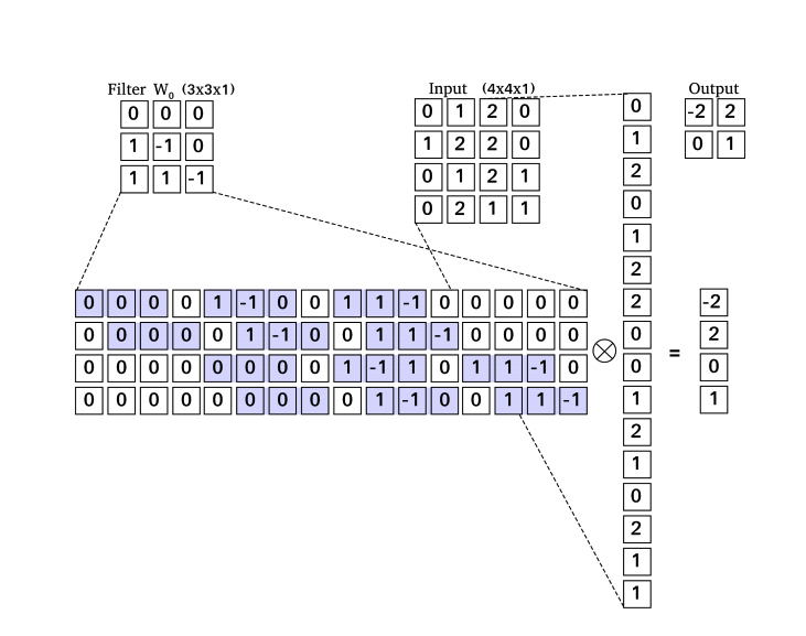
Image 3: Example of the convolution operation represented as matrix multiplication. The filter is transformed into the matrix, the input into the vector and after multiplication, we can transform the output back into the form of the output feature map.

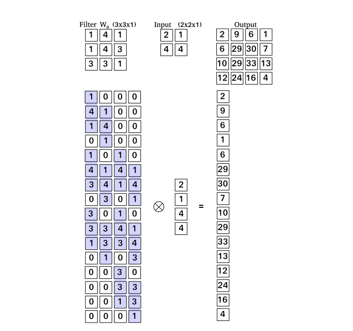
Image 4: Example of the transpose convolution  represented as matrix multiplication but with transposed filter matrix – from there name transpose convolution is derived.

Copied from Diploma Thesis with permission of author.

V Dumoulin and F Visin. A guide to convolution arithmetic for deep learning. ArXiv 1603.07285, 2016.

Augustus Odena, Vincent Dumoulin, and Chris Olah. Deconvolution and checkerboard artifacts. Distill, 2016. doi: 10.23915/distill.00003. URL http://distill.pub/2016/deconv-checkerboard.

Qifeng Chen, Jia Xu, and Vladlen Koltun. Fast Image Processing with Fully-Convolutional Networks. arXiv e-prints, art. arXiv:1709.00643, Sep 2017.

Xuaner Cecilia Zhang, Qifeng Chen, Ren Ng, and Vladlen Koltun. Zoom To Learn, Learn To Zoom. arXiv e-prints, art. arXiv:1905.05169, May 2019.

Jonathan Long, Evan Shelhamer, and Trevor Darrell. Fully Convolutional Networks for Semantic Segmentation. arXiv e-prints, art. arXiv:1411.4038, Nov 2014.

Ian Goodfellow, Yoshua Bengio, and Aaron Courville. Deep Learning. MIT Press, 2016. http://www.deeplearningbook.org.