
 Sign in
Demos & Tutorials - Gaia Users
Help supportShould you have any question, please check the Gaia FAQ section or contact the Gaia Helpdesk |
- Removed a total of (1) style font-weight:normal;
- Removed a total of (1) style margin:0;
- Removed a total of (1) align=center.
- Removed a total of (1) border attribute.
Graphical User Interface
The Graphical User Interface (GUI) of the Gaia ESA Archive offers the possibility to carry out basic and advanced queries using ADQL (Astronomical Data Query Language). The outputs of these queries can be easily downloaded in a variety of formats, including VOTable, FITS, CSV, and eCSV. Below you can find a brief description of the main features offered by the Archive, as well as two video tutorials explaining how to use it.
|
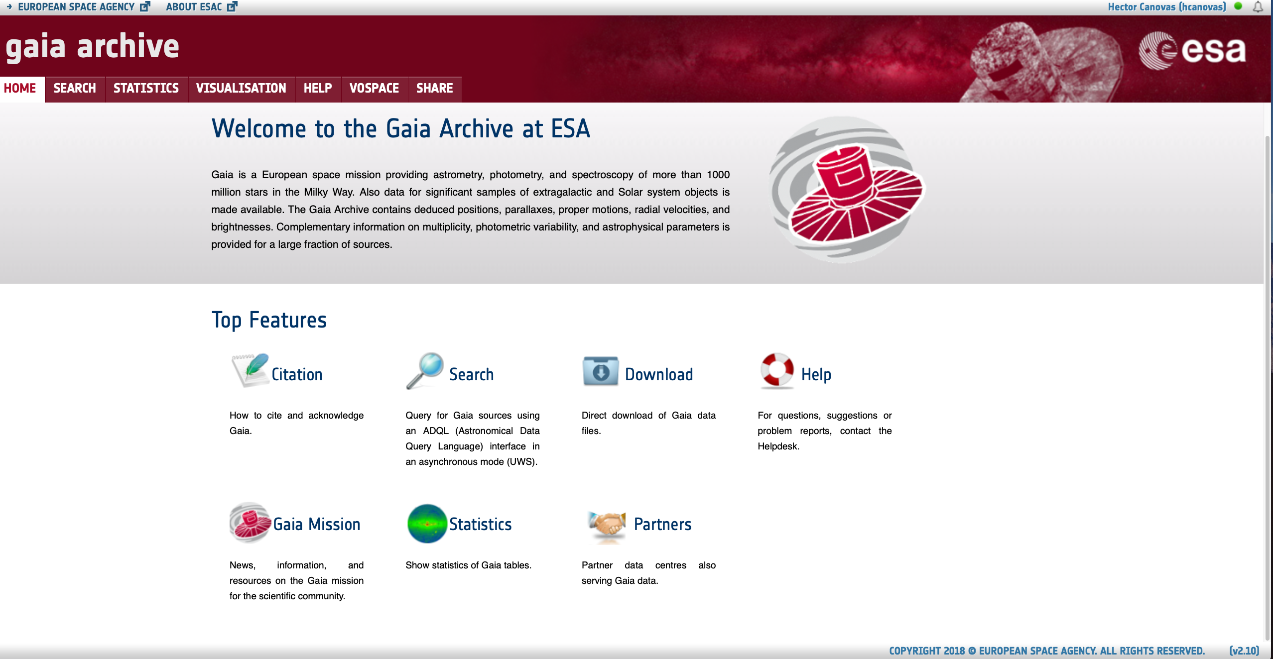
Landing pageThis is the landing page to the Gaia ESA Archive. From here, you can:
|
|
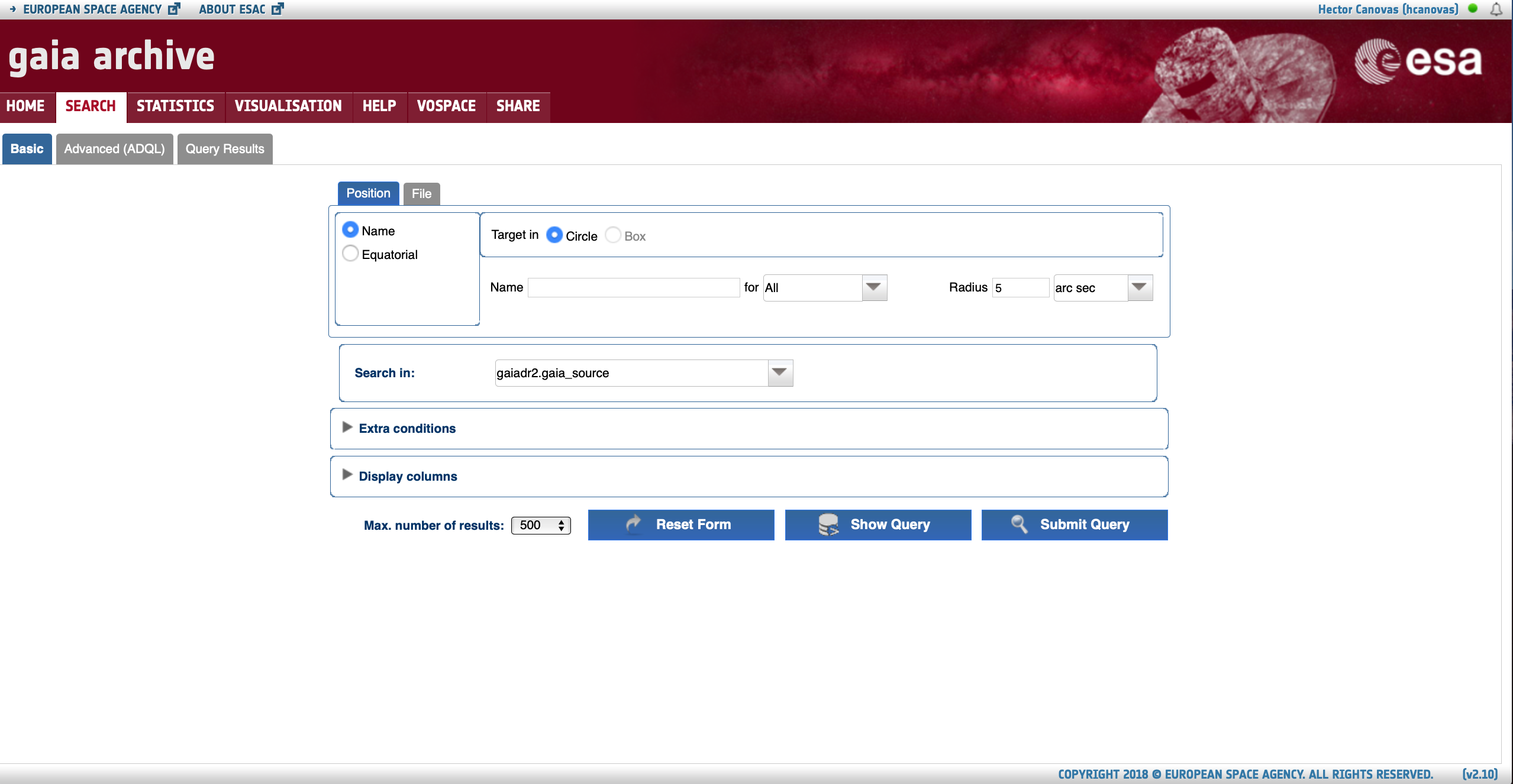
Basic query formThis form allows to easily search for data in all the catalogues hosted by the Archive. Restrictions can be added to the query using the 'Extra conditions' wizard. The output fields can be selected by means of the 'Display columns' option panel. |
|
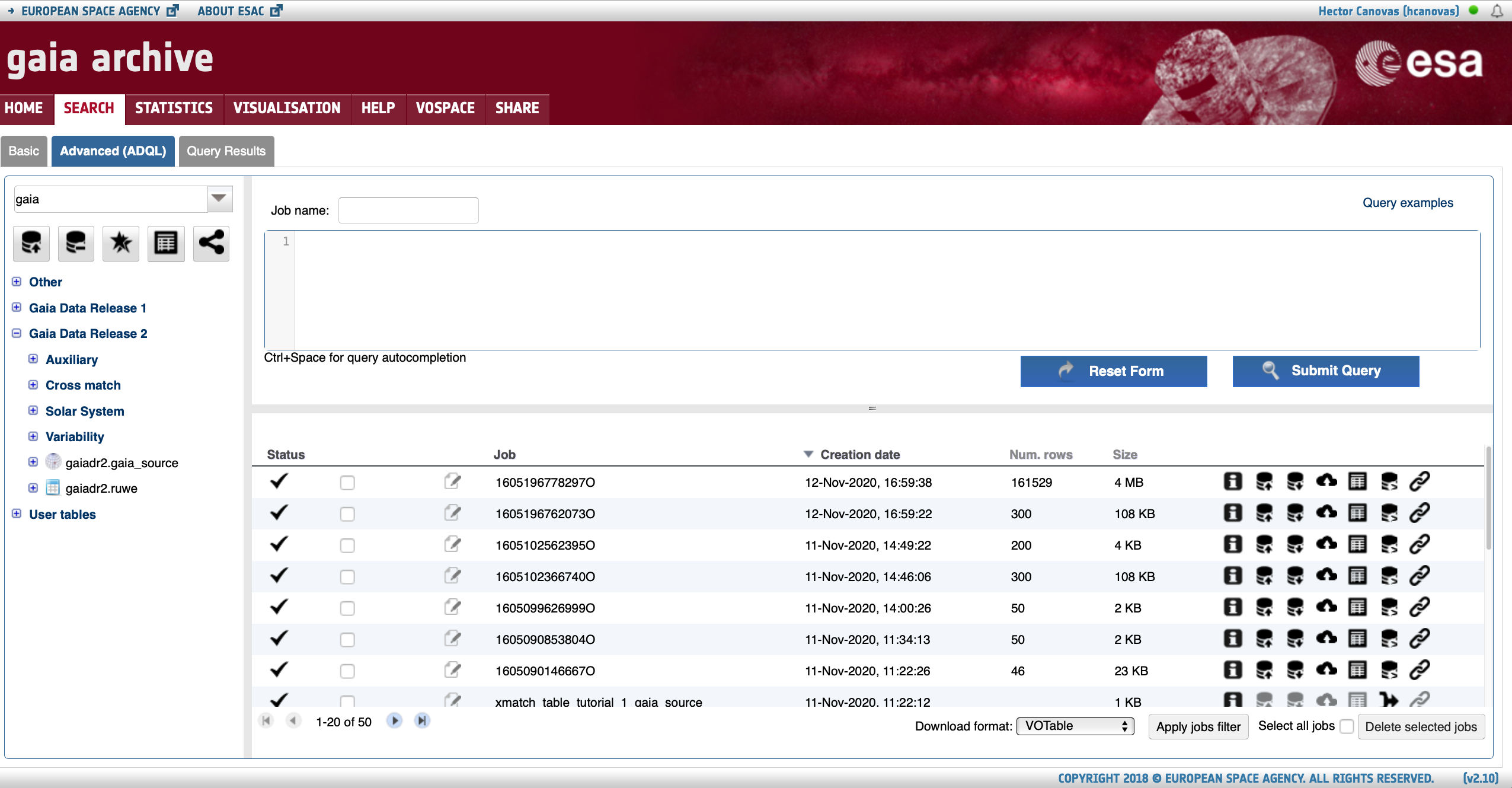
Advanced (ADQL) query formThis form allows to execute ADQL queries. Each query generates a job at the server side. The jobs executed by the user can be inspected in the list provided in this page. All the public tables and the user-uploaded tables are visible on the left side of the browser. |
|
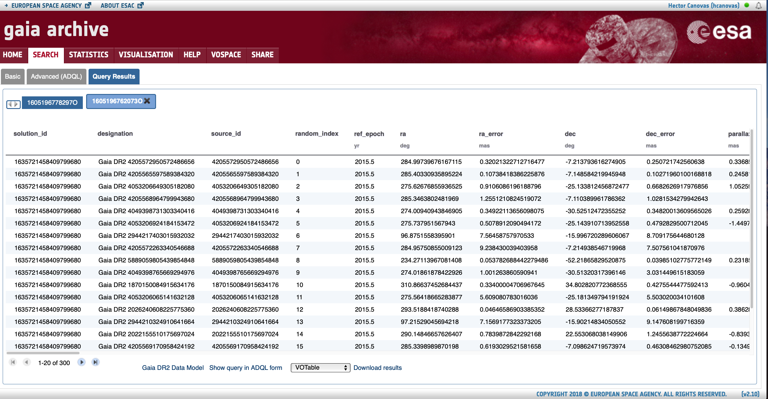
Query resultsThe output of queries are displayed in this window. The ADQL query that generated these results can be inspected by clicking on the 'Show query in ADQL form' link. |
Video: How to use the ArchiveAuthor: Deborah Baines |
Video: How to use the Archive basic formAuthor: Deborah Baines |
- Removed a total of (5) style text-align:center;
- Removed a total of (9) style text-align:justify;
- Removed a total of (1) align=left.