
 Sign in
How to extract Gaia data - Gaia Users
Help supportShould you have any question, please check the Gaia FAQ section or contact the Gaia Helpdesk |
- Removed a total of (1) style font-weight:normal;
- Removed a total of (1) style margin:0;
- Removed a total of (1) align=center.
- Removed a total of (1) border attribute.
Graphical User Interface
The Graphical User Interface (GUI) of the Gaia ESA Archive offers the possibility to carry out basic and advanced queries using ADQL (Astronomical Data Query Language). The outputs of these queries can be easily downloaded in a variety of formats, including VOTable, FITS, CSV, and eCSV. Below you can find a brief description of the main features offered by the Archive, as well as two video tutorials explaining how to use it.
|
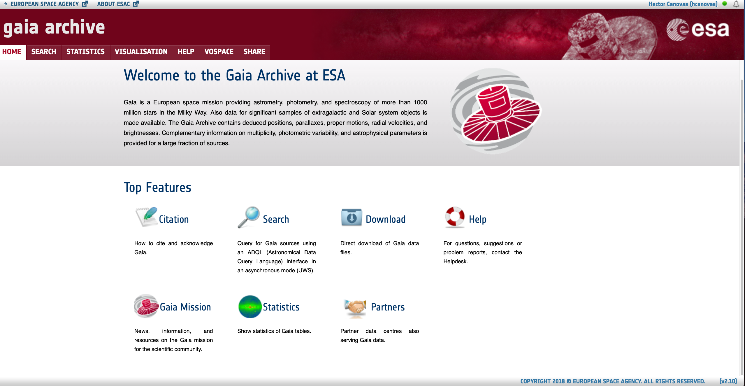
Landing pageThis is the landing page to the Gaia ESA Archive. From here, you can:
|
|
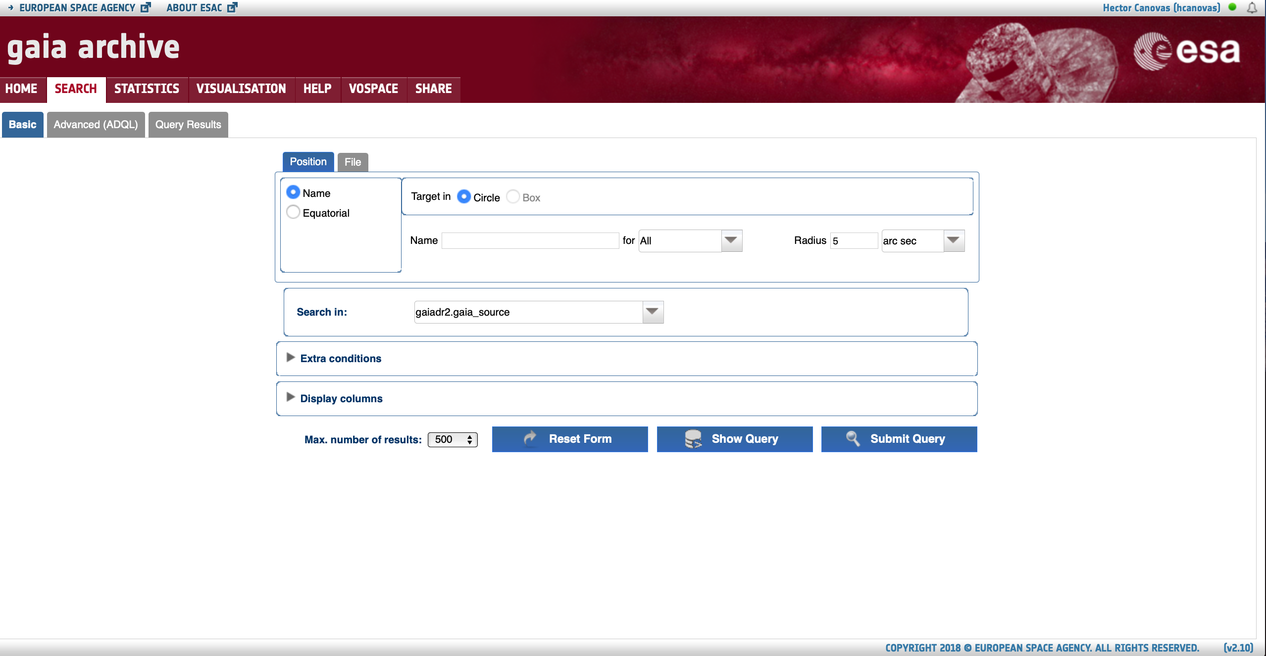
Basic query formThis form allows to easily search for data in all the catalogues hosted by the Archive. Restrictions can be added to the query using the 'Extra conditions' wizard. The output fields can be selected by means of the 'Display columns' option panel. |
|
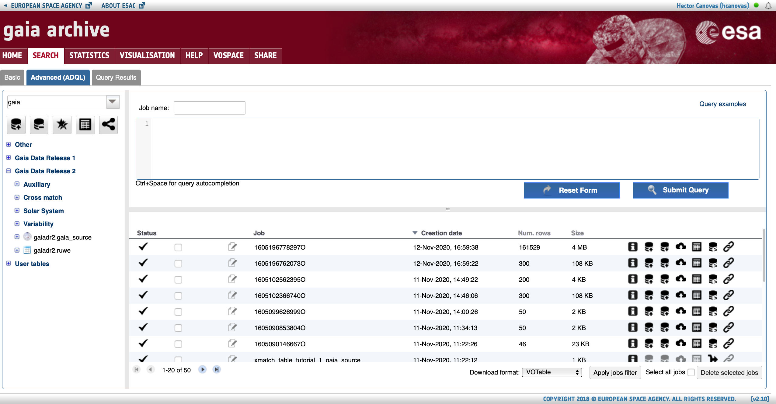
Advanced (ADQL) query formThis form allows to execute ADQL queries. Each query generates a job at the server side. The jobs executed by the user can be inspected in the list provided in this page. All the public tables and the user-uploaded tables are visible on the left side of the browser. |
|
Query resultsThe output of queries are displayed in this window. The ADQL query that generated these results can be inspected by clicking on the 'Show query in ADQL form' link. |
Video: How to use the ArchiveAuthor: Deborah Baines |
Video: How to use the Archive basic formAuthor: Deborah Baines |
- Removed a total of (5) style text-align:center;
- Removed a total of (9) style text-align:justify;
- Removed a total of (1) align=left.
Tutorial: Basic queries
Authors: Héctor Cánovas, Jos de Bruijne and Alcione Mora.
The main function of the Gaia Archive is to provide data to the astronomers. The Search tab in the GUI landing page provides two different ways of accesing the Archive for Basic (default option) and Advanced (ADQL) queries. The main objectives for the Basic tab are:
- To ease the exploration of the Archive catalogues for simple use cases, and
- To help users into the transition towards the
Advanced (ADQL)tab for complex use cases.
To that end, the Basic tab allows to perform two of the most common operations executed when exploring an astronomy archive in a very simple and intuitive manner. These operations are the ADQL cone search, which allows to search by coordinates for one or more sources in a given catalogue, and an ADQL query to retrieve all the sources encompassed by a circular or box-like region in the projected sky.
All Basic queries are synchronous, which means that they will time out after 60 and 90 seconds for non-registered and registered users, respectively (see this FAQ). Furthermore, the output of these queries is limited to 2000 sources. Therefore, we recommend to use the Advanced (ADQL) tab to execute complex and/or long queries. Through this tutorial you will learn to use the Basic tab to:
- Retrieve data for a single source.
- Retrieve data for multiple sources.
- Search for data inside a sky region.
- Understanding the query results.
1. single source data retrieval
The most basic use case could be formulated as "I want the most relevant Gaia results for a single object". It can be accomplished using the Basic > Position subtab. The first step is to fill in the "Name" box with either the object identifier (e.g. "UX Ori") or its ICRS coordinates. The accepted input formats are described in the pop-up window that appears when clicking on top of the "Name" tooltip (see Fig. 1). The single object search launches an ADQL cone search around the celestial coordinates of the input object, which are provided by the Sesame name resolver. The drop-down menu highlighted by the thin solid circle in Fig. 1 allows to choose the service that will be queried to obtain the object coordinates (by default the system tries Simbad, then NED, and then Vizier, but if the input name is a Gaia designation the system queries the Gaia Archive). Once the name or coordinates are successfully resolved the object box turns green and a confirmation message is shown. Note that epoch propagation (see this tutorial) is applied if the proper motions of the resolved source are included in the databases searched for by the name resolver. The cone search radius can be tuned using the "Radius" box, and its units can be adjusted using its associated drop-down menu (highlighted by the dashed circle in Fig. 1).
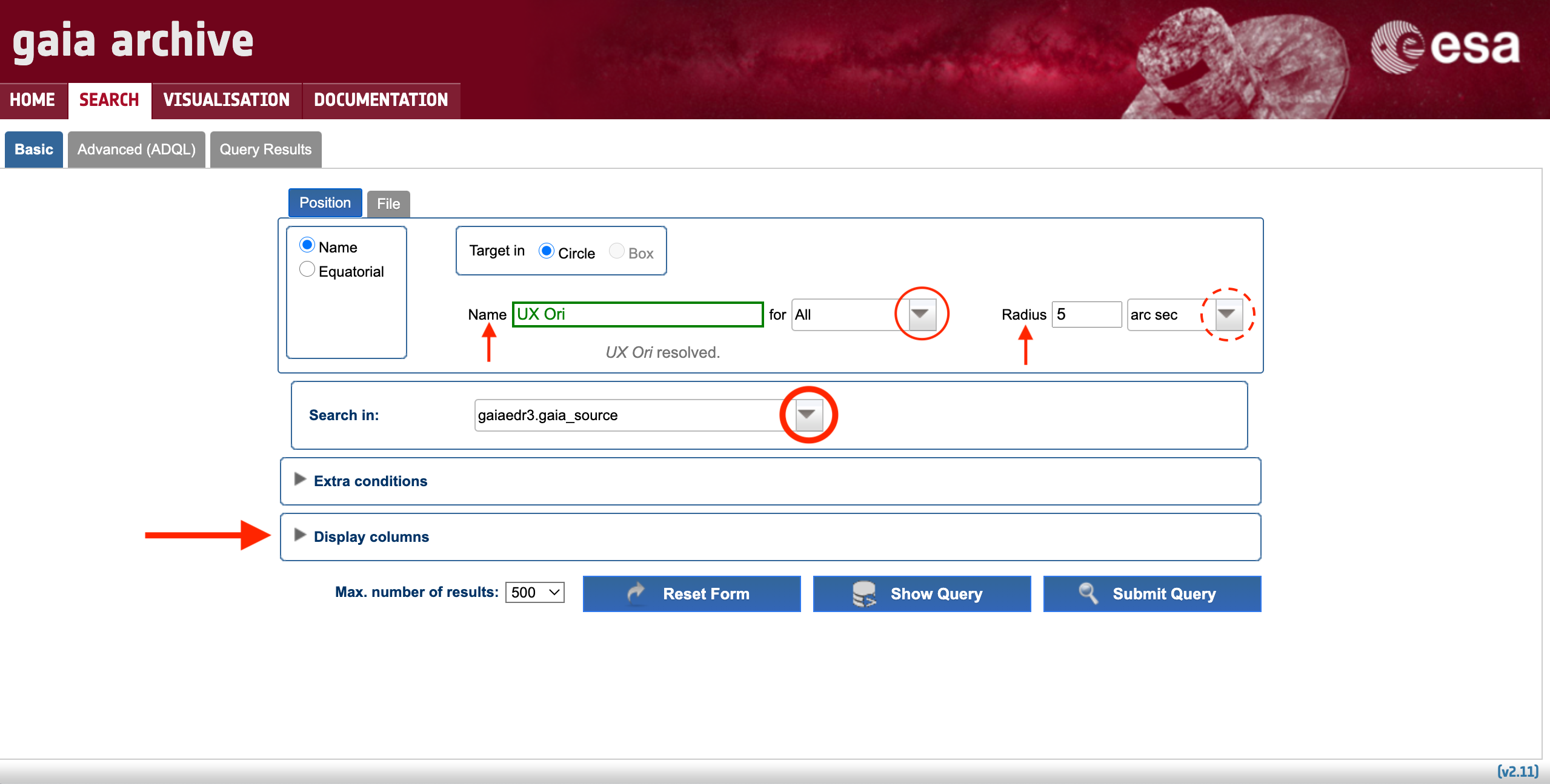
Figure 1: Content of the Basic > Position subtab (single source resolver). The vertical arrows highlight the tooltips with explanatory text, while the circles and the horizontal arrow highlight the drop-down menus and extra options available to customize the query, respectively.
The next step is to choose the catalogue that is going to be explored. The latest Gaia data release is the default one, but all the catalogues hosted by the Archive (e.g., previous Gaia data releases, external catalogues) containing geometric information in the form of celestial coordinates can be explored by clicking on the drop-down menu highlighted by the thick circle in Fig. 1. Registered users can also access to their user-uploaded tables provided that their tables contain indexed celestial coordinates (see this tutorial). By default, only a few pre-selected columns of the choosen catalogue are shown in the query outputs. Therefore, you may want to verify that the output of your search will contain the columns that you are interested in. To do so, simply click on the "Display columns" menu (indicated by the dashed horizontal arrow in Fig. 1) and mark the columns that you want to retrieve.
Now you are ready to hit the "Submit Query" button. If you are interested in learning how your query is expressed in the ADQL language, you can hit the "Show Query" button. The query results are shown in the Query Results tab, whose contents are explained in the Understanding the query results section below.
2. Multiple source data retrieval
Three common use cases are:
- I want to look for Gaia counterparts on my list of known objects,
- I want to look for the neighbours of my favourite source, and
- I want to look for the neighbours of my list of favourite sources.
2.1 Search for the Gaia counterparts of my source list
This popular use case can be accomplished using the Basic > File subtab of the GUI. First of all, you must prepare a single column ascii file (without header) with the names or ICRS oordinates of the objects you are interested in. The input file must be formatted as described in the pop-up window that appears when clicking on top of the "Select a file with Target names" tooltip (see Fig. 2). Second, select the file that you want to upload using the wizard that appears when clicking on top of the "Choose file" button. Be aware that the query output is limitted to 2000 sources. If you aim to retrieve a larger dataset you should upload your target list to your user space as explained in this tutorial, and then use the Advanced (ADQL) tab to perform a cross-match as explained in this other tutorial.
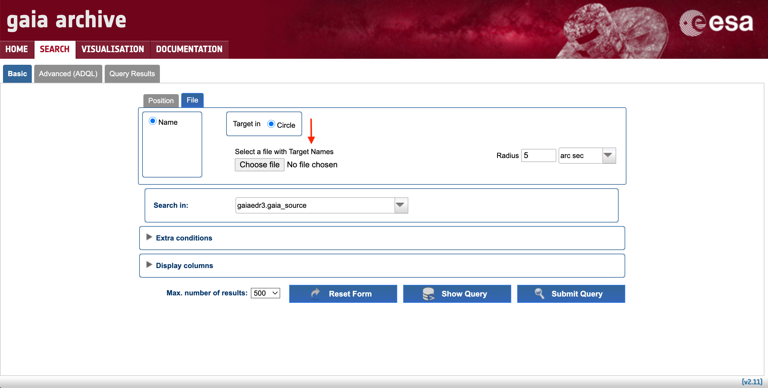
Figure 2: Content of the Basic > File subtab (multi source resolver). The arrow highlight the tooltip with explanatory text.
2.2 Search for the neighbours of my favourite source
Imagine that we want to retrieve all the sources from the Gaia EDR3 catalogue that, on-sky, are separated by less than 5 arc minutes from UX Ori. This can easily be achieved by simply updating the cone search radius units (using the drop-down menu highlighted by the red dashed circle in Fig. 1). This query outputs 195 sources, including several sources without parallax data. The Basic > Position subtab allows to apply additional selection criteria to e.g., filter out the targets with parallax signal-to-noise below a given threshold. To do so simply click on the "Extra conditions" drop-down menu as highlighted by the horizontal solid arrow in Fig. 1. A menu that allows to apply and combine different filters will show up as illustrated by Fig. 3. Applying the condition exemplified in Fig. 3 reduces the output of the previous query to 30 sources.
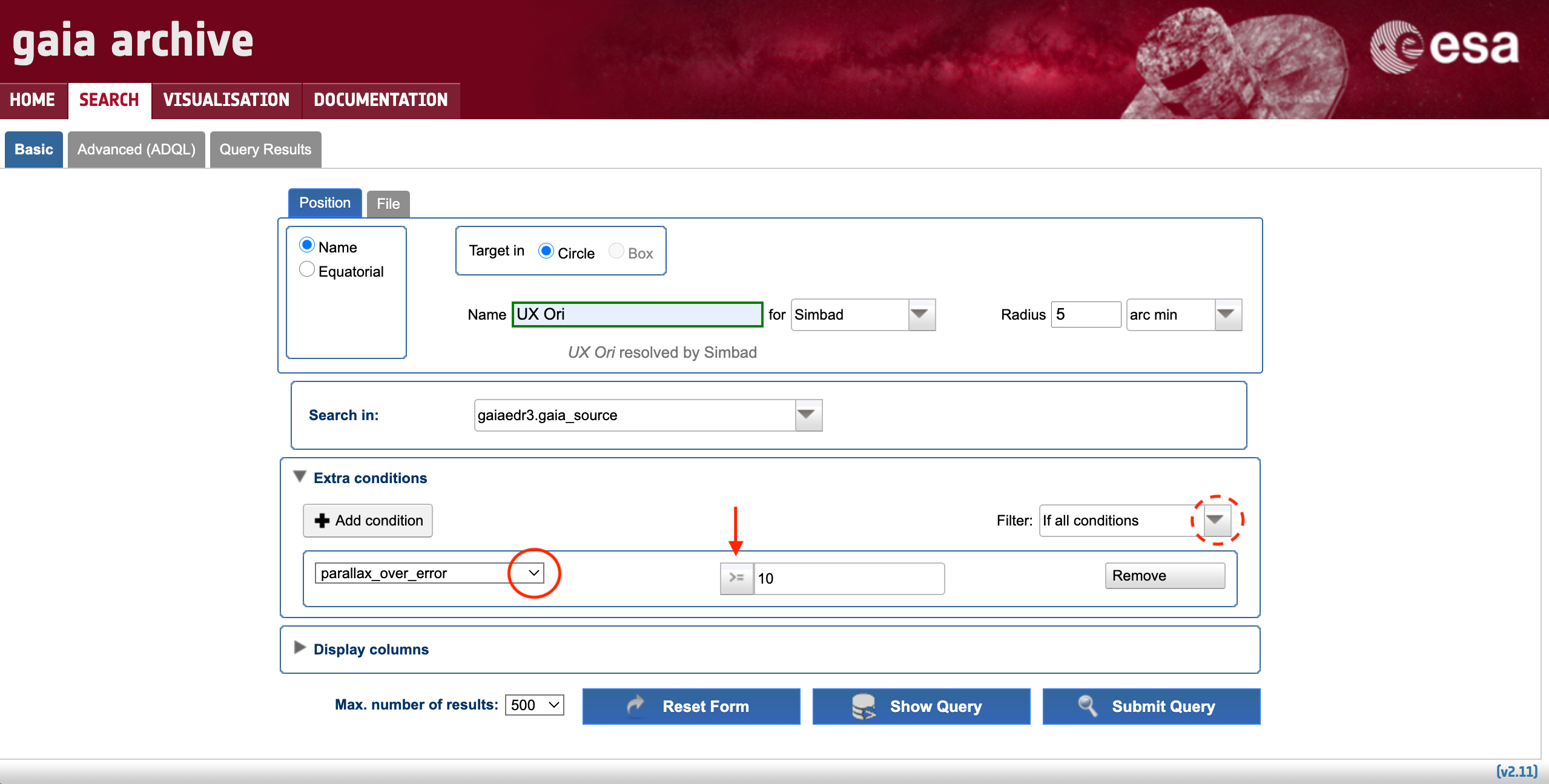
Figure 3: Content of the "Extra conditions" menu of the Basic > Position subtab. The arrow indicate how to select the operators that will be included in the query. The solid and dashed circles highlight the drop-down menus allowing to select the column over which the operator is going to be applied and the filter combination, respectively.
2.3 Search for the neighbours of my source list
This use case is a combination of the previous two cases. If you are interested in retrieving the neighbours of a pre-computed source list you should 1) upload the target list as explained in Sect 2.1 and 2) then adjust the cone search radius as described in Sect 2.2. As before, you should keep in mind that the output catalogue of the query is limitted to 2000 sources so you may want to apply a selection criteria using the "Extra conditions" menu as described in Sect 2.2.
3. Retrieve sources in a region of the sky
A cone search with an arbitrary radius can be generated around any point on the celestial sphere by entering the target coordinates in the "Name" box and adjusting the cone search radius as explained in the Single source data retrieval section. Alternatively, it is also possible to use the "Equatorial" button under the Basic > Position subtab (see Fig. 1) and choosing the "Circle" option (see Fig. 4). The Basic > Position subtab also allows to retrieve the sources encompassed by a box region in the projected sky. To do so, simply select the "Box" option, as illustrated by Fig. 4. The accepted formats of the input coordinates are described in the RA and Dec tooltips of the coordinate boxes. As with the previous options, it is also possible to add different selection criteria to filter out the query output by means of the "Extra conditions" menu.
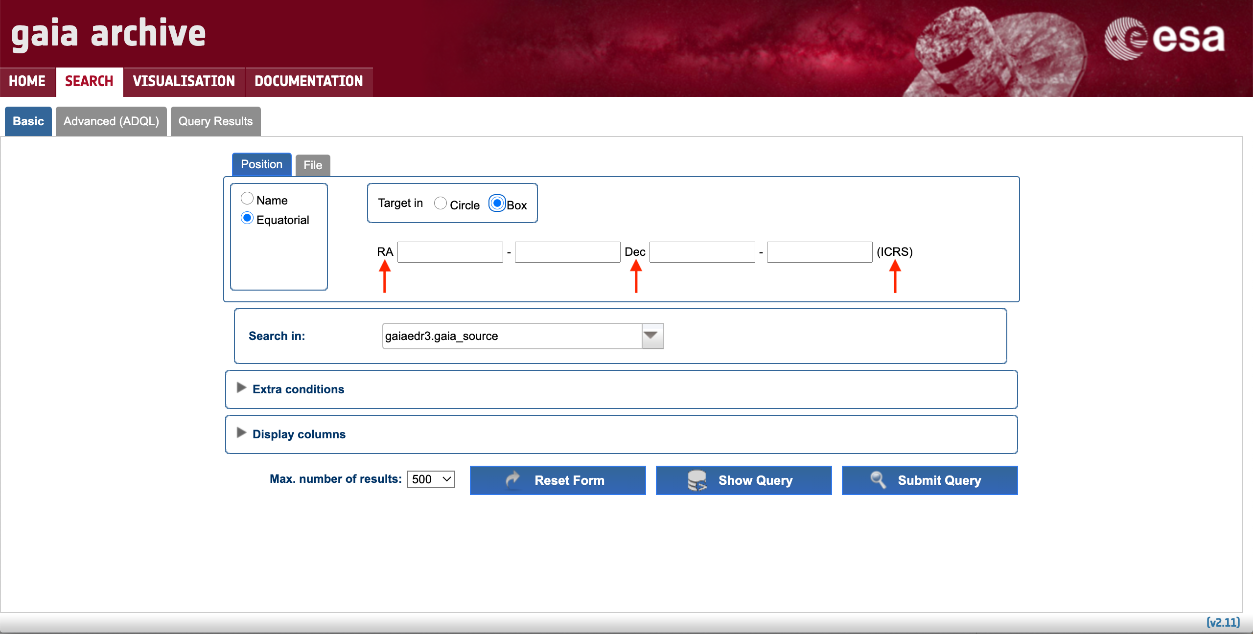
Figure 4: Content of the "Box" menu of the Basic > Position (Equatorial) subtab. The arrows indicate the tooltips with explanatory text.
4. Query Results
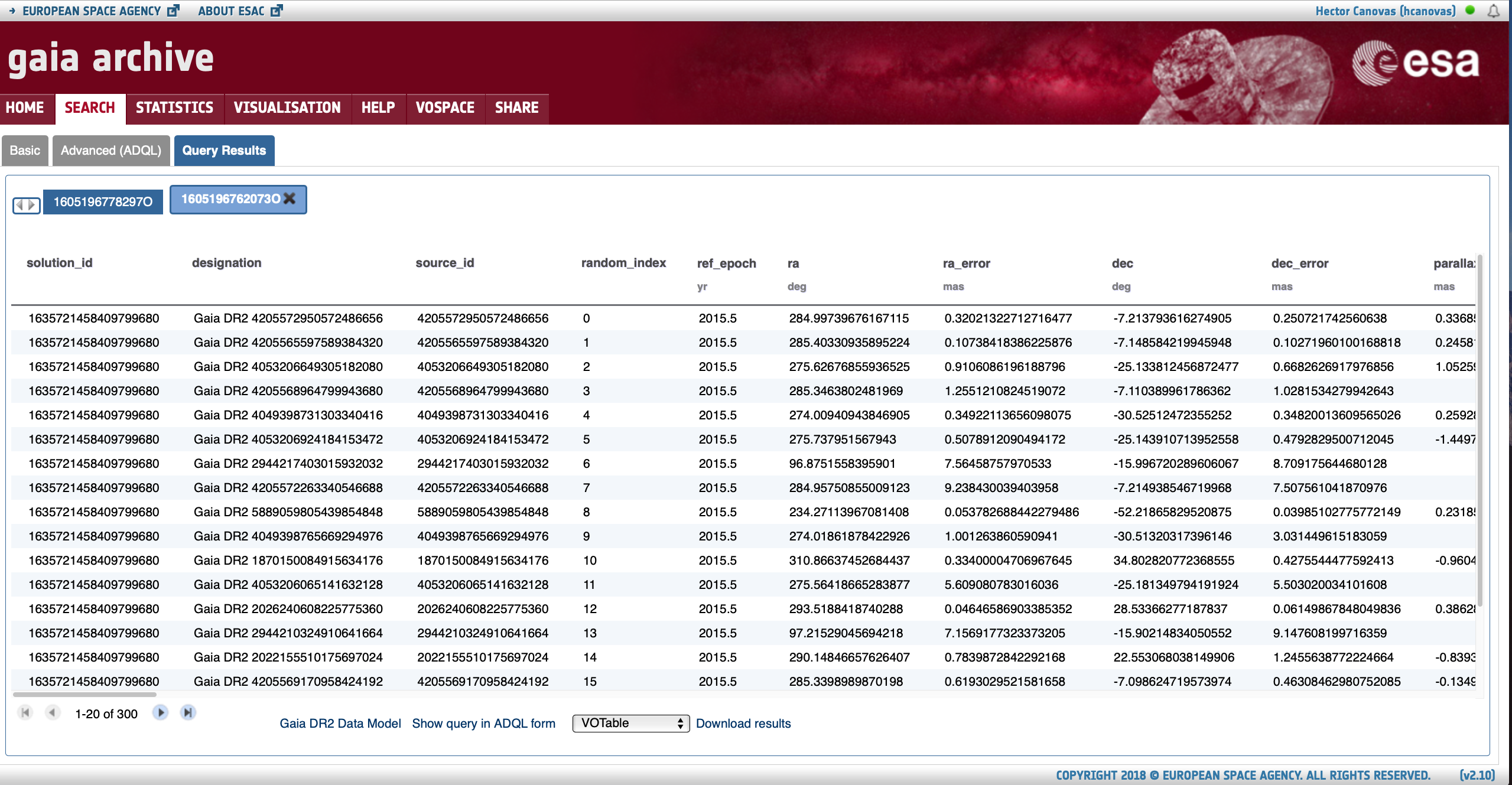
The query results are presented in tabular format in the Query Results subtab that is automatically opened once the query is finished, as shown by Fig. 5. The columns provide units when available. Further details on the meaning of each field can be found in the "<Target Catalogue> Data Model" accessible in the bottom part. Figure 5 shows the results of searching for the Gaia EDR3 counterparts of a list of sources (Sect. 2.1) and therefore the link points to the authoritative reference on the Gaia EDR3 contents. For this example only five columns ("source_id", "ra", "dec", "parallax", and "phot_g_mean_mag") were selected for displaying (using the "Displayed columns" menu as explained in Sect. 1). When the query consist in finding counterparts of an input source list in a given catalogue (as in this example), the output table contains additional columns that are automatically added by the Archive to aid the user in finding the correspondence between the input targets and the query results. These columns are:
- "target_id": contains the input target name as provided by the user in the input target list.
- "target_id, target_ra, target_dec, target_parallax, target_pm_ra, target_pm_dec, target_radial_velocity": contain data provided by the Name resolver (see Sect. 1).
- "target_distance": contains the on-sky angular separation (in units of degrees) between the target coordinates provided by the Name resolver and the target coordinates of the selected catalogue (Gaia EDR3 in this example).
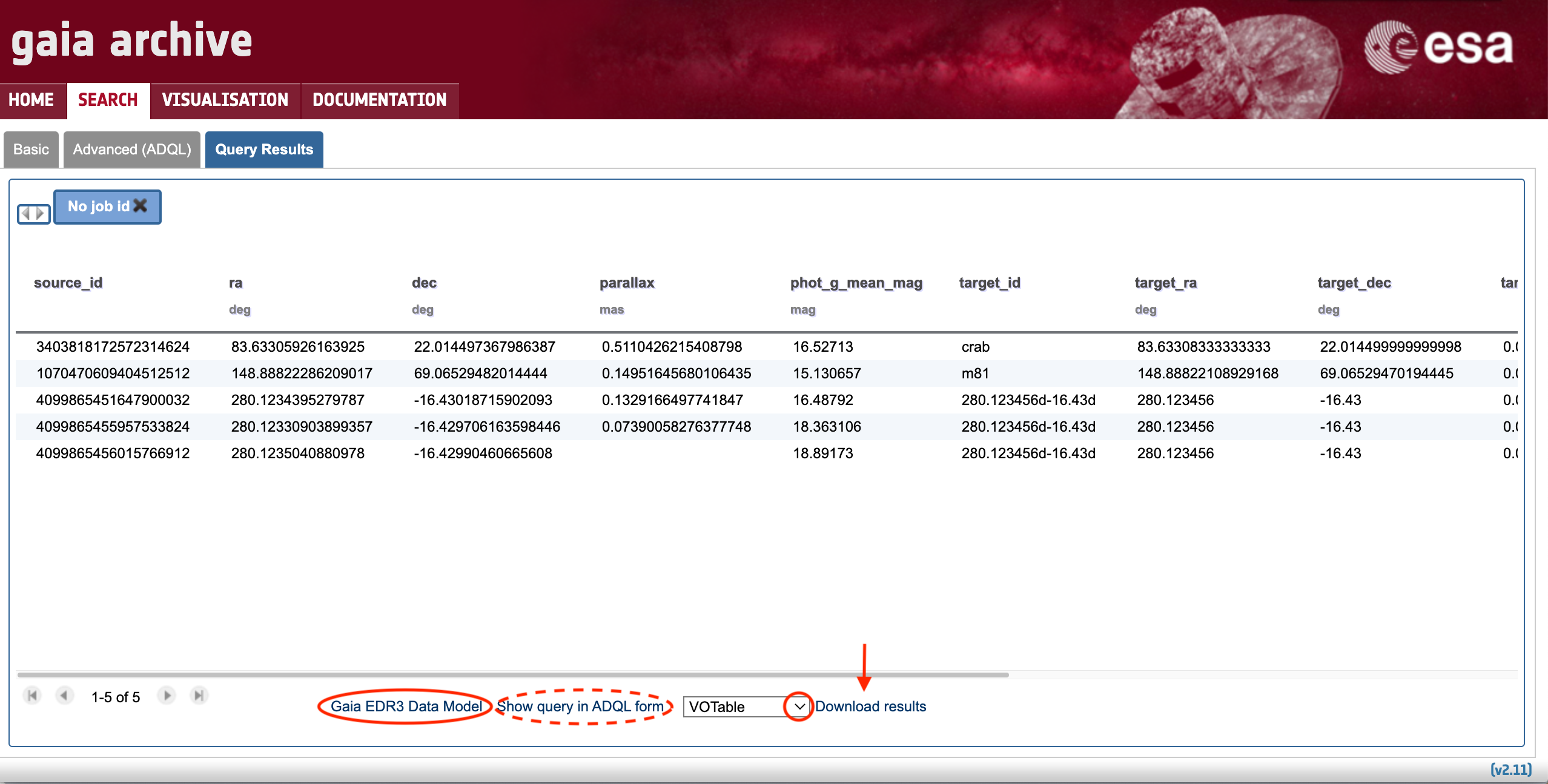
Figure 5: Query Results subtab (see text for detailed explanation). The arrows indicate the tooltips with explanatory text.
Clicking over the "Show query in ADQL form" button will open the Advanced (ADQL) tab to show the ADQL query that has been launched. This utility can be helpful for non-expert users aiming to learn the ADQL query language. Finally,the query output can be downloaded using the "Download results" menu (indicated by a vertical arrow in Fig. 5). The format of the output file can be set by means of the drop-down menu highlighted by the red circle in Fig. 5.
- Removed a total of (16) style text-align:center;
- Removed a total of (38) style text-align:justify;
Tutorial: Advanced (ADQL) tab
Authors: Héctor Cánovas & Alcione Mora
The Advanced (ADQL) form of the GUI allows to execute complex ADQL queries, inspect the Archive catalogues, upload tables to the user space, and take advantage of a number of utilities developed by our team to facilitate the exploration and scientific exploitation of the Gaia Archive. All Advanced (ADQL) queries are asynchronous, which means that they will time out after 90 and 120 minutes for non-registered and registered users, respectively (see the "Why does my query time out after 90 minutes? Why is my query limited to 3 million rows?" FAQ). The output of these queries is limited to 3,000,000 sources for non-authenticated users, whereas it is unlimited for authenticated ones. The Advanced (ADQL) tab is divided in three main areas that are highlighted in Fig. 1.:
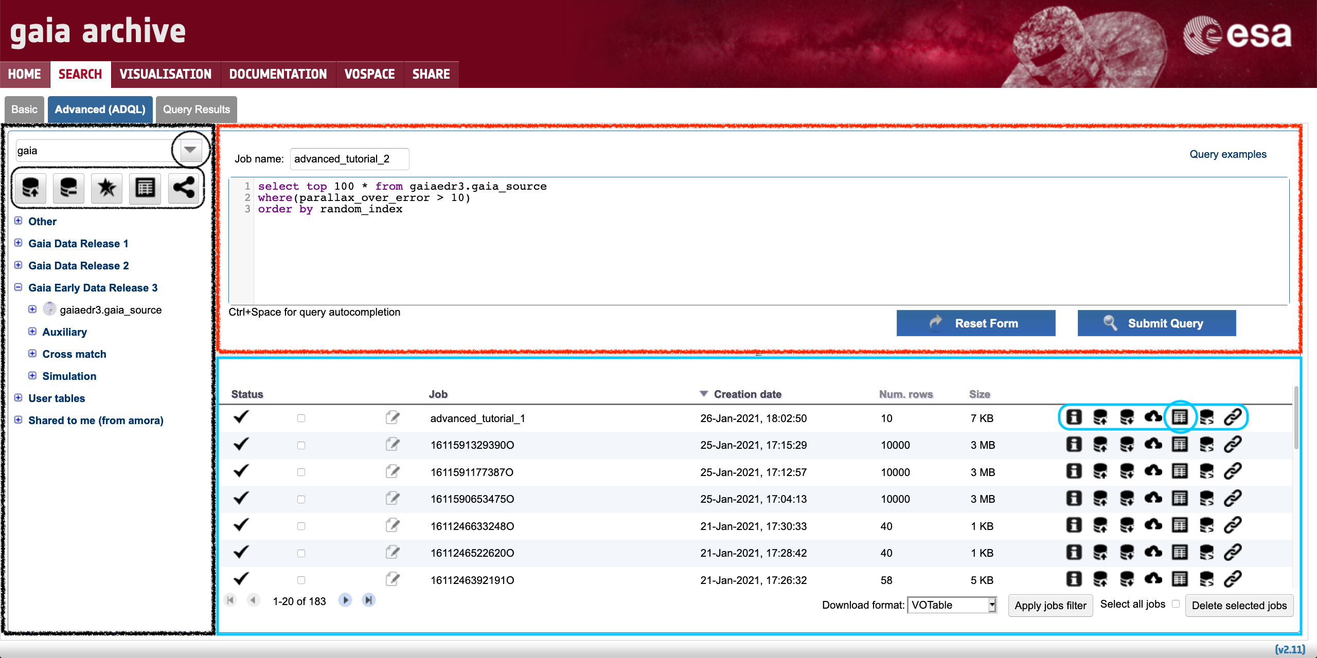
Figure 1: Content of the Advanced (ADQL) tab. The large red-wrinkled and blue-solid rectangles encompass the ADQL query editor and Jobs list areas, respectively. The large black rectangle contains the tables tree.
1. The ADQL query editor
This box allows to introduce ADQL queries to explore the catalogues hosted by the Archive. Many of the most common types of queries that are executed in the Archive (like cone searches, cross-matches, or computing the proper motion propagation of a given sample of objects) can be loaded by clicking on top of the "Query Examples" text (see Fig. 1). All these examples, along with a basic explanation and a reference (when appropriate) can also be found under the "Writting Queries/Query Examples" section of the left-side menu of this page. For more information and references about the ADQL language please take a look at the "Writting queries/ADQL syntax" section of that menu. Pressing the "Submit Query" button launches the query, which in turn generates a "job" in the Archive. A job has several attributes, including the results that contain the output of the launched ADQL query. The job ID can be specified before launching the query using the "Job name" box. This utility helps reminding the goal of a given query when visiting the Archive in the future. The job results are presented in a tabular form and - once a job succesfully finishes - they can be examined by clicking on top of the table-like icon located in the Jobs list (highlighted by the red circle in Fig. 1). This action will show up a table in the Query Results tab (see the "Understanding the Query Results" section of this tutorial to learn more details about the content of this tab).
2. The jobs LIST
Each row of the Jobs list contains relevant information about the jobs previously launched, like:
- The status (a job can be succesfully finished, failed, or it can be under execution),
- The job ID (either an alpha-numeric code assigned by the Archive or a user-defined name),
- The creation date,
- The number of rows of the job result, and
- The size of the job result.
The jobs launched by registered users are stored in their accounts, which have a job quota limit of 2 GB. The number of jobs stored in an account is shown at the bottom left of the page (in the example shown in Fig. 1 there are 183 jobs stored). This number appears surrounded by two pair of arrows that allow to navigate through the job list. The expandable menu "Apply jobs filter" allows to select jobs executed within a given range of time, as well as to filter out jobs by their status (e.g., completed, aborted, executing, etc.) Jobs can be deleted by means of the "Delete selected jobs" option. Additionaly, the Jobs list contains 7 buttons (encompassed by the small blue rectangle in Fig. 1) that, from left to right, allow to:
- Obtain detailed job information,
- Export the job result to a table and upload it to the user account (see this tutorial for details),
- Download the job result as a table (the file format of the downloaded file can be set using the "Download format" menu),
- Upload the job result to the user VOspace,
- Examine the job result in the
Query Resultstab, - Show the ADQL query that generated the job in the ADQL parser, and
- Explore the datalink products (if any) associated to the job results.
3. The tables tree
The tables tree allows to directly access to all the catalogues hosted by the Archive. These catalogues are organised under different branches that can be expanded by clicking on the "+" sign next to each schema name (see Fig. 2). A first look at this box shows that the tables have three different types of associated icons. Tables having indexed celestial coordinates are marked with an spherical-like icon, and they can be explored within the Basic query tab (see Fig. 1 in this tutorial). The tables lacking indexed coordinates column are marked with a table-like icon, while the cross-matches between two tables are marked with a double-star like icon. Clicking on top of a table name will open a pop-up window with basic information about the table. From that window it is also possible to directly show the first 20 rows of the table, which will open in the Query Results tab. Clicking on the "+" sign next to each table name will expand the table content to show its column names. Indexed columns appear with bold fonts, and the (indexed) primary key of the table appears in bold red fonts.
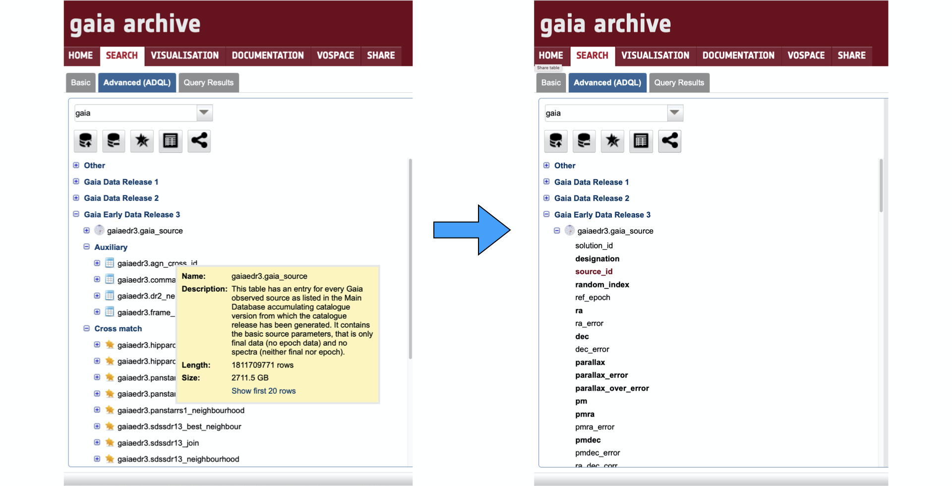
Figure 2. Left: Selected content of the Catalogue box. The yellow pop-up window appears after clicking on top of the table name. Right: Content of the "gaiaedr3.gaia_source" catalogue, that is revealed by clicking on top of the "+" sign next to the table name.
From left to right, the five buttons placed on top of the catalogue schemas (encompassed by the small black rectangle in Fig. 1) allow to:
- Upload a local table to the user space (see more details about this utility in this tutorial),
- Remove a table from the user space,
- Run a positional cross-match between two tables,
- Edit the table properties, and
- Share a table with the members of a given group (see this tutorial for more information about the sharing capabilities of the Archive).
Furthermore, it is possible to easily combine the catalogues and tables hosted by the Gaia Archive with other catalogues hosted by external TAP services. To access to this advanced utility click on top of the arrow encompassed by the black circle as indicated in Fig. 1. This dedicated tutorial explains how to make use of this this powerful functionality.
- Removed a total of (7) style text-align:center;
- Removed a total of (13) style text-align:justify;
Advanced Archive Features
Authors: Héctor Cánovas, Jos de Bruijne, and Alcione Mora
The Gaia ESA Archive is based on the Virtual Observatory Table Access Protocol (TAP), which allows to retrieve data from astronomical databases using ADQL queries. The Archive offers a number of powerful functionalities for advanced users, as presented in this tutorial.
Tutorial content:
- JOB UPLOAD
- Download data from an external TAP server
- TAP_UPLOAD: Run queries in an external TAP server
- Common table expressions: WITH
- Set operators (UNION, EXCEPT, INTERSECT)
1. Job_Upload
This mechanism allows to run a query against a job that already exists in the Archive, using the unique alpha-numeric code assigned to each job (the job ID, as explained in Sect. 2 of this tutorial). For example, let us assume that we have retrieved a sample of Gaia DR2 sources encompassed by a 1 degree radius circle centred in HL Tauri, located in the Taurus star forming region, as follows:
SELECT source_id, ra, dec, pmra, pmdec, parallax, phot_g_mean_mag
FROM gaiadr2.gaia_source
WHERE DISTANCE(POINT(67.91046, 18.23274), POINT(ra, dec)) <1. AND parallax_over_error > 10.
The job associated to this query will appear in the job list area of the Advanced (ADQL) tab of the Archive. In our case, it is job ID "1696340111393O". Having this information at hand, it is easy to identify the Gaia EDR3 sources matched to the output of the previous query using the pre-computed Gaia EDR3 - Gaia DR2 cross-match table ("gaiaedr3.dr2_neighbourhood" - see Chapter 10 of the Gaia EDR3 online documentation) as follows:
SELECT intermediate.*, dr3Xdr2.*
FROM job_upload."job1696340111393O" AS intermediate
JOIN gaiaedr3.dr2_neighbourhood AS dr3Xdr2 ON dr3xdr2.dr2_source_id = source_id
2. Download data from External TAPs
There are many TAP services around the globe (an extensive list of TAP servers can be found here). This section explains how to discover, explore, and combine data from external TAPs within the Gaia Archive, which implements the Global TAP Schema (GloTS) maintained by GAVO. Advanced users may also use the excellent TAP client TOPCAT to retrieve data from different TAP servers.
Imagine we want to combine HST/ACS photometry from the NGC 346 open cluster analysed by Gouliermis+ (2006) with Gaia data. The first step is to look for this resource. First, once in the Advanced (ADQL) tab of the Archive, we need to click on the scrollable menu showing "gaia" on top of the tables tree, and then in "External TAP search" as indicated in Fig. 1 below:
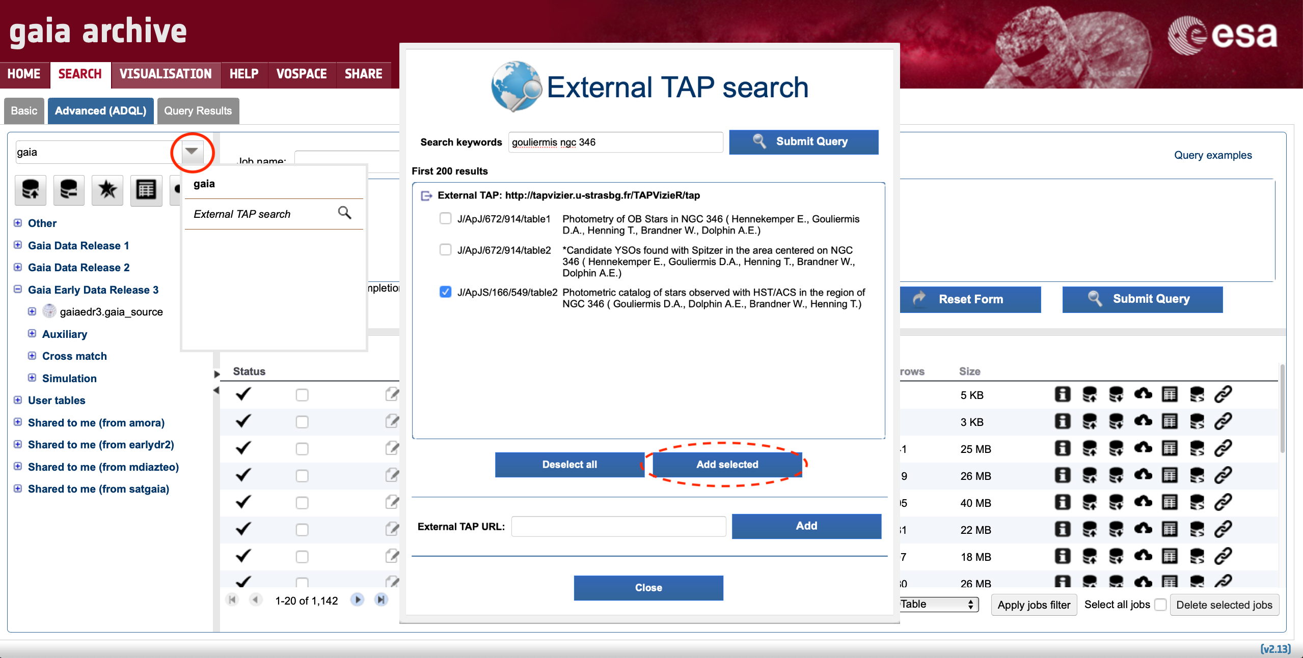
Figure 1: Screenshot of the Advanced (ADQL) tab showing how to use the external TAP search functionality. First, click on the downwards arrow encompassed by the red circle. After selecting "External TAP search", a pop-up window appears on the screen. In this example, introducing "gouliermis ngc 346" in the "Search keywords" box shows 3 TAP tables, all of them hosted by the VizieR TAP service at CDS. The content of these tables can be visually inspected by selecting them and clicking on top of of the "Add selected" button encompassed by the red ellipsoid.
After clicking on "Add selected", the Archive is instructed to send future requests to the external TAP of our choice (in this example that would be the TAP VizieR service at CDS). At this stage, standard ADQL commands can be entered in the Gaia Archive user interface while these commands will be run at CDS. For example, the following query retrieves the entire Gouliermis+ (2006) catalogue:
SELECT * FROM "J/ApJS/166/549/table2"
When selecting an external TAP, the Advanced (ADQL) tab interface changes as illustrated by Fig. 2 to highlight that only the external TAP tables are accessible at this time. This means that, in addition to the selected table, all catalogues hosted by the TAP service of the external data centre can be queried using the ADQL query editor on the Gaia Archive, provided we know the table name (and associated field names) of the external catalogue. For example, the following query will retrieve the first 10 entries from the Spitzer C2D legacy catalogue (Evans et al. 2009):
SELECT TOP 10 * FROM "J/ApJ/672/914/table2"
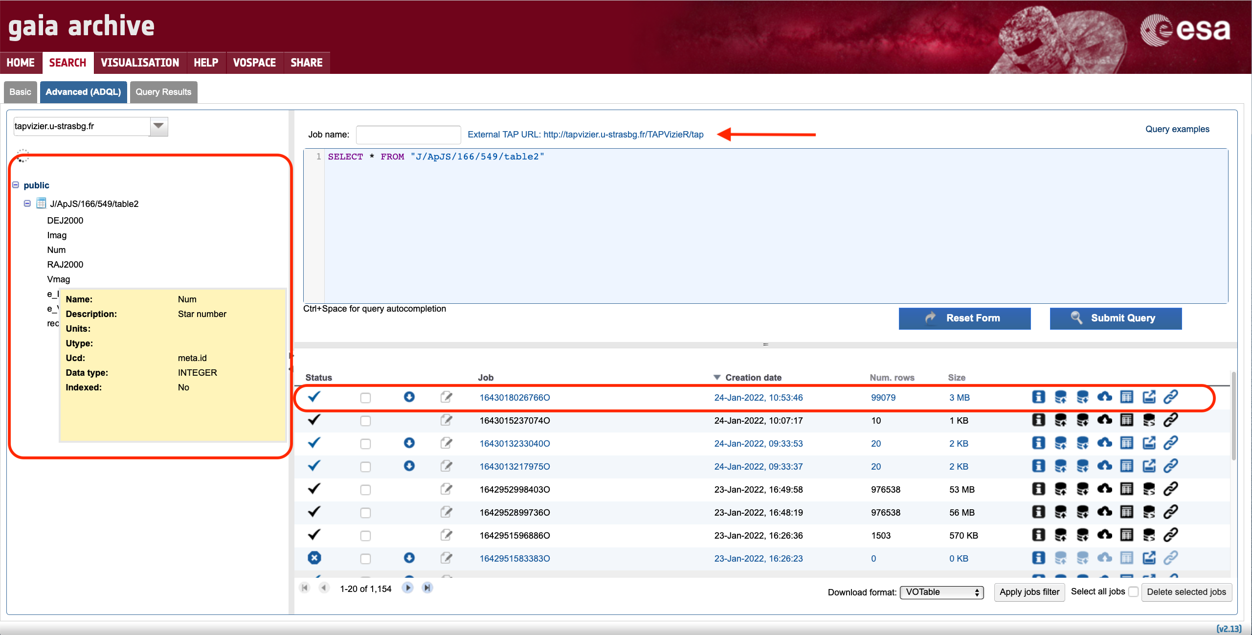
Figure 2: Screenshot of the Advanced (ADQL) tab showing the interface changes that appear when the Gaia Archive is connected to an external TAP server: 1) the tables tree only displays the selected table in the previous step (see Fig. 1), 2) the ADQL query editor background adopts a "blueish" colour and the external TAP url is shown on top of the editor, and 3) the executed jobs are displayed in the job list using blue fonts.
In order to stop the connection to the external TAP server, simply click on the drop-down menu on top of the table tree (see red circle in Fig. 1) and select "gaia".
The typical workflow for using external catalogues requires the combination (join) of the externally retrieved data with those hosted in the Gaia Archive. One possibility is uploading the table to the user space, as explained in the "Upload a user table" tutorial. For small catalogues, or those to be used only once, it is also possible to use JOB_UPLOAD functionality as explained in Sect. 1.
3. TAP_UPLOAD: Run queries in an external TAP
Sometimes the combination goes in the opposite direction. Imagine that we want to complement the dataset created in Sect. 1 above with the CATWISE 2020 photometry that is available in the VizieR TAP server. As a first step, we can find the catalogue following the steps listed in Sect. 2 above and searching for keyword "catwise". Once the external TAP connection is established, our dataset can be uploaded and included in the query using the TAP_UPLOAD.<job_id> ADQL feature as follows:
SELECT upload.*, catwise.*
FROM tap_upload.job1641568769115O AS upload
JOIN "II/365/catwise" AS catwise
   ON 1 = CONTAINS(POINT('ICRS', catwise.RA_ICRS, catwise.DE_ICRS), CIRCLE('ICRS', upload.ra, upload.dec, 1. / 3600.))
*Notes:
- The VizieR TAP server requires that the first element of the POINT & CIRCLE functions is an string. Additionaly, these functions are optimised differently than in the Gaia Archive, as the coordinates of the larger (smaller) catalogue should be placed in the POINT (CIRCLE) function to obtain optimal performance.
- The tap_upload mechanism does NOT requires using double quotation marks enclosing the target job_id.
4. Common table expressions: WITH
The WITH feature can be used to simplify the syntax of of nested queries, in a similar manner than the job_upload mechanism described in Sect. 1 above. For example the Positional Xmatch+proper motion propagation example can be re-written as follows:
WITH subquery AS (
     SELECT gaia.*, ESDC_EPOCH_PROP_POS(ra, dec, parallax, pmra, pmdec, radial_velocity, ref_epoch, 2000) AS propagated_position_vector
     FROM gaiadr3.gaia_source AS gaia
     WHERE DISTANCE(POINT(56.75, 24.12),POINT(gaia.ra, gaia.dec)) < 5.0 AND
    SQRT(POWER(gaia.pmra - 20.5, 2) + POWER(gaia.pmdec + 45.5, 2)) < 6.0)
SELECT subquery.source_id, subquery.parallax, subquery.phot_g_mean_mag, galex.*
FROM subquery
JOIN external.galex_ais AS galex
  ON DISTANCE(POINT(COORD1(subquery.propagated_position_vector), COORD2(subquery.propagated_position_vector)),
              POINT(galex.raj2000, galex.dej2000)) <1./3600
Note, however, that this simplification comes at the cost of lower performance (a factor of ~2-3) compared to the nested query described in the Positional Xmatch+proper motion propagation example. Note that splitting the query into two separated queries with the second one making use of the job_upload mechanism is usually the most efficient option in terms of total execution time.
5. Set operators (UNION, EXCEPT, INTERSECT)
The ADQL 2.1 set operators (UNION, EXCEPT, INTERSECT) allow to concatenate vertically the outputs of different queries as long as the outputs have the same number of columns (and they have identical names). The example below shows how to retrieve the DR3 data contained in two overlapping, circular (radius = 0.15 degrees) regions separated by ~0.2 degrees around Baade's Window (ra, dec = 270.89, -30.03 deg) using these operators (replacing <SET_OPERATOR> by UNION, UNION ALL, EXCEPT, or INTERSECT):
SELECT * FROM gaiadr3.gaia_source
WHERE DISTANCE(POINT(270.89, -30.03), POINT(ra, dec)) < 0.15 <SET_OPERATOR> SELECT *
FROM gaiadr3.gaia_source
WHERE DISTANCE(POINT(270.89, -30.24), POINT(ra, dec)) < 0.15
Executing the first part of the query alone produces a table with 81,061 rows while runing the full query using the set operators produces the following output sizes:
- Removed a total of (4) style text-align:center;
- Removed a total of (7) style text-align:left;
- Removed a total of (14) style text-align:justify;
- Removed a total of (1) style font-weight:bold;
- Removed a total of (2) style overflow:auto;
- Removed a total of (2) style margin:0;
- Removed a total of (2) style display:block;
Tutorial: Bulk Download
Authors: Héctor Cánovas, Jos de Bruijne, Enrique Utrilla, and Alcione Mora
Although most of the Archive ADQL queries only require accessing small portions of the Gaia catalogue table(s), a number of users need to work with a full catalogue or a significant fraction of it. In those cases, analysing the data locally is probably more efficient than using the Gaia ESA Archive. Chopping a large table into small chunks to sequentially download them using a bash or a Python script is possible (see the Programmatic Access section), but this approach is prone to errors (like, e.g., those created by unexpected network glitches) and very expensive in terms of execution time. This is the reason why all the tables stored in the Gaia ESA Archive are also available for direct download in the Gaia ESA Archive bulk download repository (sometimes referred to as content delivery network or CDN). We strongly recommend users to retrieve the files from this directory if they are interested in storing locally (a large fraction of) the complete catalogue. This tutorial describes the content of the bulk download directory, including code to download the files contained in selected sky regions.
Directory structure
Gaia (E)DR3
The content of the entire gaia_source table is partitioned in multiple files based on 3386 ranges of HEALPix level-8 indexes (as illustrated by Fig. 1 below). In this way, each file (except for the last one) contains around 500,000 sources. There is one file for each of those ranges, identified by a suffix containing the first and the last HEALPix level-8 indexes included in it (except if the range contains no source at all, in which case no file is generated). For example, the file "GaiaSource_000000-003111.csv.gz" contains all Gaia DR3 sources encompassed between HEALPix level-8 indices 0 and 3111. The same partitioning has been applied to all the tables in the (E)DR3 release, with the following exceptions:
- the tables that do not have a source_id field, i.e., total_galactic_extinction_map, total_galactic_extinction_map_opt, oa_neuron_information, and oa_neuron_xp_spectra, are very small and are each stored in a single file;
- the tables that do have a source_id field but have few entries (such as gaia_crf3_xm, science_alerts, and alerts_mixedin_sourceids) are each stored in a single file;
- the solar-system object (SSO) tables are split into 20 files.
Several tables that have been published in the Gaia EDR3 release are also applicable to Gaia DR3. These include pre-computed cross-match tables, simulated data, and the commanded scan law. These tables have not been duplicated in the DR3 repository but can be downloaded from the EDR3 repository.
For detailed information about the generation of these files, please read the Data Consolidation chapter in the Gaia DR3 documentation. For maximum compatibility, all files are plain text files in Enhanced Character Separated Value format (ECSV) format, compressed with the standard GZIP algorithm. ECSV files are regular CSV files, with an extra header with metadata about the table itself and its columns in YAML format, preceded with the "#" comment character.
Gaia DR2
The content of the tables is partitioned in the same way as in the Gaia (E)DR3 case described above. However, in Gaia DR2 the file names contain the minimum and maximum source_id included in each file (instead of HEALPix index). For example, the file "GaiaSource_1000172165251650944_1000424567594791808.csv.gz" contains all Gaia DR2 sources encompassed between source_ids 1000172165251650944 and 1000424567594791808. For Gaia DR2, all files are plain text files in CSV format, compressed with the standard GZIP algorithm.
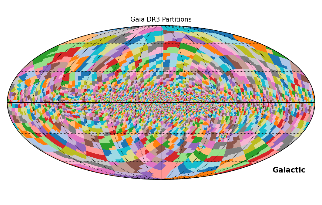
Figure 1: Sky coverage of the 3386 partitions applied to the gaia_source catalogue in (E)DR3, in Galactic coordinates.
Files download
The bulk download repository contains several complementary .txt files that should be read carefully before downloading any dataset. Those include the "_disclaimer.txt" and "_citation.txt" files as well as the "_catalogue_sizes.txt" file that contains information about the total size of each (compressed) table. The uncompressed files can be up to ~10 times larger than the compressed ones (depending on the file contents). In addition, each (catalogue) directory contains an "_MD5SUM.txt" file that can be used to verify that the retrieved dataset has not been corrupted while downloading and/or saving the files.
entire catalogue
As explained in this FAQ, the "wget" command is a useful tool to download catalogues from the Gaia Archive bulk download directory. The following example shows how to retrieve the entire EDR3 gaia_source table:
wget --recursive --no-parent 'http://cdn.gea.esac.esa.int/Gaia/gedr3/gaia_source/'
Partial download (cone-search alike)
As explained above, the Gaia (E)DR3 files have their associated minimum and maximum HEALPix level-8 indexes included in their names. By construction, a HEALPix index represents a selected area in the projected sky and it is possible to recover the central coordinates of this region using diffent tools available in the literature (like the Astropy-healpix package). The notebook below takes advantage of this information and utilities to identify all the files that contain sources in a circular region of the sky. In practice, it does something similar to an ADQL cone-search operation, but targeting the user-selected files stored in the bulk download directory. This notebook is convenient for users aiming to download large fractions of the Archive catalogues. This code has been tested in Python >= 3.8. The Jupyter notebook is included in this .zip file that also contains complementary notebooks, supplementary files, and a "tutorials.yml" environment file that can be used to create a conda environment with all dependencies needed to execute it (as explained in the official conda documentation). The file also includes a similar notebook but adapted to download Gaia DR1 and DR2 data.
Cone search > Bulk download
Release number: v1.1 (2022-08-06)
Applicable Gaia Data Releases: Gaia EDR3, Gaia DR3
Author: Héctor Cánovas Cabrera; hector.canovas@esa.int
Summary:
This code computes the list of Gaia (E)DR3 files associated to a circular region in the sky defined by the user. The granularity of this region is set by the HEALPix level selected.
Input parameters:
- target catalogue (e.g., gaia_source, auxiliary/agn_cross_id, or auxiliary/frame_rotator_source),
- the cone-search parameters (centre and radius), and
- the desired healpix level.
Once the variables above are set the notebook creates a reference file that contains the min/max HEALPix index (levels: 6,7,8, and 9) encompassed by each gaia_source file available in the (E)DR3 bulk download directory.. The convertion between the different HEALPix levels is done by means of bit-shifting operations.
Useful URLs:
import os
from datetime import datetime
import numpy as np
import pandas as pd
from astropy import units as u
from astropy_healpix import HEALPix
Set input variables
Default input paramers:
- DR3 = True ; Default Value. Set it to False to retrieve EDR3 files
- target_table = 'gaia_source' ; Alternative values: 'Astrophysical_parameters/astrophysical_parameters', 'Variability/vari_cepheid', etc - see all the content in: http://cdn.gea.esac.esa.int/Gaia/gdr3/ & http://cdn.gea.esac.esa.int/Gaia/gedr3/
- Cone-search parameters: radius = 0.5 degrees, centred in the Large Magallanic Cloud (in ICRS coordinates).
- Healpix-level = 6 (choose a larger one to increase granularity, and viceversa).
# Set input parameters below ===========
DR3            = True            # Set it to False to select EDR3
target_table   = 'gaia_source'   # Alternative values: 'Astrophysical_parameters/astrophysical_parameters/', etc
hpx_level      = 6
lon            =  80.894 * u.deg # Right Ascencion (ICRS)
lat            = -69.756 * u.deg # Declination (ICRS)
radius         = 0.5     * u.deg
print(f'Input Variables: ')
print(f'* HEALPix level                      = {hpx_level} ')
print(f'* ICRS longitude (~ Right Ascension) = {lon} ')
print(f'* ICRS latitude  (~ Declination)     = {lat} ')
print(f'* Radius                             = {radius} ')
print()
# Download basic parameters ============
output_file    = 'bulk_download_files.txt'
output_dir     = 'downloads'

if os.path.isdir(f'{output_dir}'):
   now = datetime.now()
   output_dir_2 = output_dir + now.strftime("_%Y-%m-%d")
   print(f'>> Warning: {output_dir} directory exist. Creating alternative directory: {output_dir_2}')
   print()
   output_dir   = output_dir_2
else:
   os.system(f'mkdir {output_dir}')

print(f'Files will be downloaded to: {output_dir}')
Create reference file
if DR3:
   gaia_dr_flag = 'DR3'
else:
   gaia_dr_flag = 'EDR3'

print('='*120)
print(f'Preparing selection of Gaia {gaia_dr_flag}: ""{target_table}" files')
print('='*120)

url_prefix      = f'http://cdn.gea.esac.esa.int/Gaia/g{gaia_dr_flag.lower()}/{target_table}/'
md5sum_file_url = url_prefix + '_MD5SUM.txt'
md5sum_file     = pd.read_csv(md5sum_file_url, header=None, delim_whitespace=True, names=['md5Sum', 'file'])

if DR3:
   md5sum_file.drop(md5sum_file.tail(1).index,inplace=True) # The last row in the "_MD5SUM.txt" file in the DR3 directories includes the md5Sum value of the _MD5SUM.txt file
md5sum_file
# Extract HEALPix level-8 from file name ======================================
healpix_8_min  = [int(file[file.find('_')+1:file.rfind('-')])     for file in md5sum_file['file']]
healpix_8_max  = [int(file[file.rfind('-')+1:file.rfind('.csv')]) for file in md5sum_file['file']]
reference_file = pd.DataFrame({'file':md5sum_file['file'], 'healpix8_min':healpix_8_min, 'healpix8_max':healpix_8_max}).reset_index(drop=True)

# Compute HEALPix levels 6,7, and 9 ===========================================
reference_file['healpix7_min'] = [inp >> 2 for inp in reference_file['healpix8_min']]
reference_file['healpix7_max'] = [inp >> 2 for inp in reference_file['healpix8_max']]

reference_file['healpix6_min'] = [inp >> 2 for inp in reference_file['healpix7_min']]
reference_file['healpix6_max'] = [inp >> 2 for inp in reference_file['healpix7_max']]

reference_file['healpix9_min'] = [inp << 2       for inp in reference_file['healpix8_min']]
reference_file['healpix9_max'] = [(inp << 2) + 3 for inp in reference_file['healpix8_max']]

# Generate reference file =====================================================
ncols          = ['file', 'healpix6_min', 'healpix6_max', 'healpix7_min', 'healpix7_max', 'healpix8_min', 'healpix8_max', 'healpix9_min', 'healpix9_max']
reference_file = reference_file[ncols]
reference_file
Compute Healpix indexes associated to the selected circular region
print('='*120)
print(f'Computing HEALPix Level {hpx_level} encompasing a Cone Search (Radius, longitude, latitude): {radius.value} {radius.unit},  {lon.value} {lon.unit}, {lat.value} {lat.unit}')
print('='*120)

hp             = HEALPix(nside=2**hpx_level, order='nested')
hp_cone_search = hp.cone_search_lonlat(lon, lat, radius = radius)
Download files
A .txt file with the list of files to be downloaded will be firts created. This file will be read and a secuencial download of all the files listed will start. A progress message will be in the terminal from where this Notebook was launched.
f = open(output_file, "w")

subset     = []
for index in reference_file.index:
    row = reference_file.iloc[index]
    hp_min, hp_max = row[f'healpix{hpx_level}_min'], row[f'healpix{hpx_level}_max']
    if np.any(np.logical_and(hp_min <= hp_cone_search, hp_cone_search <= hp_max)):
       bulk_file = url_prefix + row['file'] + '\n'
       f.write(bulk_file)
       subset.append(bulk_file)
f.close()

print('='*120)
print(f'A total of {len(subset)} files for download were written in {output_file}')
print('='*120)
print('='*120)
print(f'Bulk download files are stored in directory: {output_dir}')
print('='*120)
os.system(f'wget -i {output_file} -P {output_dir}/ -q  --show-progress --progress=bar:force 2>&1')
- Removed a total of (2) style text-align:center;
- Removed a total of (2) style text-align:right;
- Removed a total of (23) style text-align:justify;
- Removed a total of (1) style float:right;
- Removed a total of (2) style margin:0;
- Removed a total of (1) align=right.
- Removed a total of (2) border attribute.