Neural Network

In 1943 the first formal model of an artificial neuron was proposed by McCulloch and Walter Pitts. Their neuron worked like a logic gate. The neuron acted as OR, AND, NOT logical operations; thus enabled the network to act like a computer. The model lacked an essential feature – learnable weight. In 1950s Frank Rosenblatt introduced a perceptron. In this model, neurons were connected by variable weights: the output is one of the weighted sums of its input is above threshold, and zero if it is below. The first implementation of the perceptron was not by software, because it was prolonged back then. Rosenblatt decided to build his device were weights were implemented by variable resistors, and learning the weights was done by electric motors that turned the knobs on the resistor [Domingos, 2018].

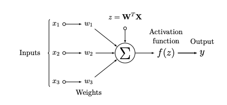
Image 1: Scheme of neuron

The fundamental principle of the neural network is usually compared with the basic block of our brain – neuron. The basic unit of the neural network is called a neuron. Every neuron n is connected trough weighted connection w_n (Image 1). Input x_n is multiplied by weight wn and sum up

Equation 1

where b_n is a bias which helps to improve the performance of the network. Because in neural networks, one is usually dealing with a large number of inputs, and weights, it is convenient to write Equation 1 in matrix multiplication form, where bias is inserted into weight (W), and input (X) matrix on the zero position

 Equation  2

Next step is application of an activation function on output y = f(z) . The activation function is an important part of the neural network; without it the neural network would work like a linear transformation of its input. The function introduces non-linearity to the network. If we want to create the neural network we need to put basic units, neurons, in hierarchy structures – layers. The first layer is called the input layer, it takes our training data. The following layers are hidden layers. The number of hidden layers, and neurons in it, are optional. We can choose how big network we want to create depending on our problem.

The input layer contains input data. The input information goes to the first hidden layer where matrix multiplications are done; then the output is used as an input for the second hidden layer etcetera. The output layer, the last layer of the network, contains the output information, e.g. our input belongs to class A or class B.

In the beginning, the neural network weights are initialised randomly to non-zeros small values. This values must be different; otherwise, training of the network would fail. During the training of the network, the information goes from the input layer through hidden layers to the output layer. After the last layer, a loss function is used to evaluate the performance of the network. The loss function calculates an error of the output. The last step is the backpropagation; errors are propagated to the network, and weights are changed [Goodfellow et al., 2016, Raschka, 2015] .

Basic terminology

Some of the terms commonly used in ML field.

The activation function

The activation function is the nonlinear transformation that we do over the signal f(z), transformed output is then sent to the next layer of neurons as input. Without an activation function, a neural network would do a linear transformation.

The loss function

The loss or cost function (L) measures a quality of trainable parameters and how they should be updated. The goal is to minimize the loss function by changing weights and biases.

Backpropagation

Back-propagation is the learning process, which propagates the error through the network. It computes the derivatives of a loss function and changes the weights of the parameters. Sets of weights in every layer are represented by matrices, but the last layer generates a vector. In forward pass, we derive the matrix first and then we multiply it with next matrix. That can be computationally expensive. The algorithm computes gradient in backward order – gradient of the output layer is calculated first. If we derive first the output vector and multiply with a matrix in the next layer, then it yields another vector. That is the reason why is the back-propagation computationally efficient approach. Back-propagation can be summarized into three steps: 

1. Output vector is computed.

2. Result is compared with true labels and loss is computed.

3. Weights are updated via back-propagation.

Copied from Diploma Thesis and Bachelor Thesis with permission of author.

Pedro Domingos. The Master Algorithm: How the Quest for the Ultimate Learning Machine Will Remake Our World. Basic Books, Inc., USA, 2018. ISBN 0465094279.

Ian Goodfellow, Yoshua Bengio, and Aaron Courville. Deep Learning. MIT Press, 2016. http://www.deeplearningbook.org.

Sebastian Raschka. Python Machine Learning. Packt Publishing, 2015. ISBN 1783555130.