Tools for simulations - Athena

Tools for simulations

For scientific simulation activities please use the responses available through the X-IFU and WFI Consortia web pages.

Newathena mirror Requirement implementation

The NewAthena mirror requirements are implemented through the following mirror configuration:

Mirror Assembly (MA) with 13 rows, 6 sectors, 492 mirror modules
Active mirror apertures radius 245-1120 mm
Mirror plate rib spacing (pitch) of 2.27 mm
10 nm of Ir coating on each individual module, plus 8 nm C (top) and 12 nm Cr overcoating. The CrC layer thickness has been optimised to achieve the best possible area at low and high energies (unpublished study by Desiree della Monica Ferreira, DTU)
0/+2 wedging geometry

The mirror geometry will be described in the Athena Telescope Reference Document (TRD) version 3.4 by the ESA Study Team.

Component Data Files: area and on-axis PSF

Estimates of the on-axis effective area and vignetting curves have been calculated by ESA using SIMPOSiuM (Sironi et al., 2021, SPIE, 11822, oOM), an advanced and innovative end-to-end X-ray tracing code developed specifically to predict the performance of the Silicon Pore Optics (SPO) technology on Athena. a They have been based on realistic ray-trace experiments including all known loss effects. In addition, they do include provisional loss factors to account for expected losses such as misalignments, coating imperfections, contamination, etc. The simulations correspond to the simulated mission at beginning-of-life conditions.

Point Spread Function (PSF) parameterization and images have been extrapolated by ESA from estimates originally provided by Prof. Richard Willingale (University of Leicester).

NewAthena mirror peformance resources

Mirror Effective Area On-Axis (1 eV energy resolution): NewAthena_mirror_effectiveArea_IrCCr_13rows_v1.1.dat
Vignetting as a function of energy (0.2, 0.35, 1, 2, 4, 7, and 10 keV) and off-axis angle (0, 0.5, 1.0, 2.0, 3.0, 5.0, 7.0, 10.0, 15.0, 20.0, 28.0 arcminutes): NewAthena_vignetting_13rows_v1.dat
Parameterization of the PSF as a function of energy (see above) and off-axis angle (0, 2, 6, 12, 20, 28 arcminutes): na_psf_vig_hew_9_13rows.dat. The PSF model is a 2-D distribution whose radial profile corresponds to a modified pseudo-Voigt distribution.
On-axis PSF images as a function of energy (E) and off-axis angle (a) (see above): NA_HEW9.tar.gz. They correspond to a nominal pixel size of 0.1".

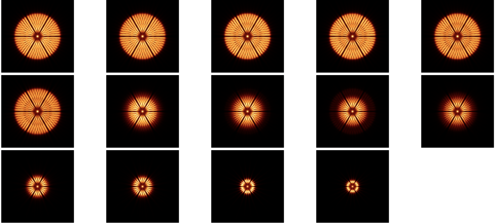
ATHENA ON-AXIS De-focused PSF images

Images (FITS) of the 35-mm de-focused PSF of the Athena mirror (800x800 pixels, pixel size=0.25") at: 0.2 keV, 0.35 keV, 0.75 keV, 1 keV, 1.25 keV, 1.5 keV, 2.5 keV, 3 keV, 4 keV, 6.5 keV, 7 keV, 10 keV, 12.5 keV. They are based on recent analytical calculations (May 2021) improving the accuracy of prior estimates.

X-ray stray light

This tarfile contains software (C procedure) and associated data files to produce stray light estimates (credit: Prof. Richard Willingale, University of Leicester). They will be shortly integrated in SIXTE to produce images directly usable for scientific simulations.