
 Sign in
Intermediate Data - Hipparcos
Intermediate Data |
|||||||||||||||||||
|
This app plots barycentric and observed positions (with error bars) for a requested star using the Hipparcos intermediate astrometric data; some statistical charts are also generated for the data. |
 |
||||||||||||||||||
Main plot |
|||||||||||||||||||
|
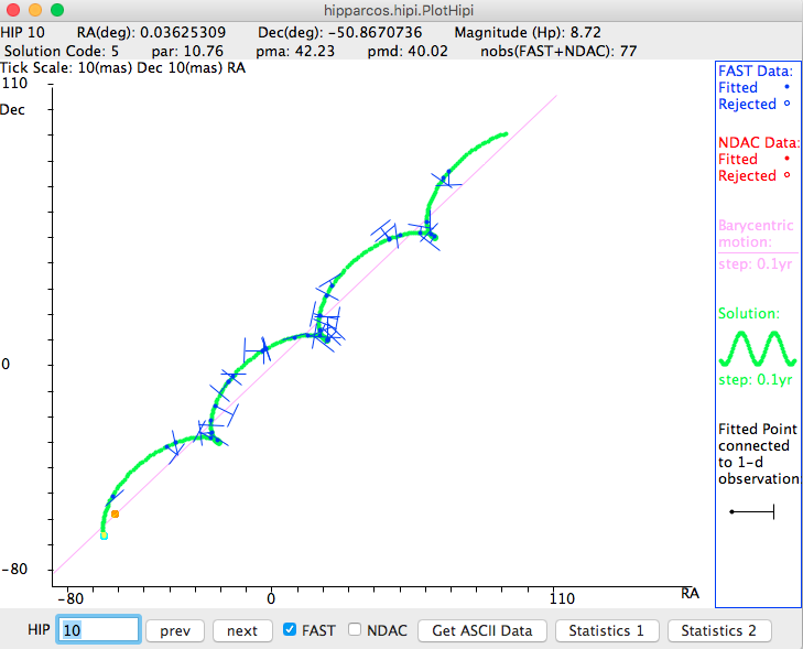
The main plot shows the path on the sky of the requested Hipparcos Catalogue object, covering the actual span of observations, typically amounting to a period of about three years centred around the adopted mean Catalogue epoch of J1991.25. Equal scales are adopted in both RA and Dec; this scale allows the observations to fill the window, irrespective of the magnitude of the astrometric parameters: thus the relative size of the error bars will appear larger for objects with small values of parallax and proper motion, and vice versa. In practice, the error bars are mainly dependent on the magnitude of the object. |
|||||||||||||||||||
|
|||||||||||||||||||
| The individual observations are shown as blue (FAST) or red (NDAC) points (either, both, or neither can be activated: if neither are displayed, the plot shows simply the adopted solution; this facility may be useful in the case of fainter stars with larger residuals, or in the case of objects with small numerical values of the parallax and proper motion, e.g., HIP 1, 5, etc.). Observations rejected from the fit (usually none) are shown as open circles. Further details of these data points are given below. The straight line shows the barycentric motion of the object, from which only the proper motion of the object is apparent, i.e., it shows the (solved) motion of the object as viewed from the solar-system barycentre, without the effect of parallax. The continuous curve is the modelled stellar path fitted to all of the (accepted) measurements, based on the astrometric parameters given in Catalogue Fields H8-9 and H11-13 (the curve is generated using an approximate Earth ephemeris, resulting in an rms positional error of about 0.0024 AU over the interval 1988.0 to 1993.0). The amplitude of the oscillatory motion gives the star's parallax, with the linear component representing the star's proper motion. The FAST/NDAC data points are shown as follows. Solid circles indicate the inferred position of the object at each observation epoch. By definition, these fitted points lie on the continuous modelled path. A straight line (the residual of each observation) joins the fitted point to the observed position line of the star at the relevant epoch. Because the measurement is one-dimensional, the precise location along this position line is undetermined by the observation. The position line (always perpendicular to the residual line) is shown with a length of +/-5 milliarcsec, although the true uncertainty in this dimension is considerably larger (in effect it is unconstrained by the observations). Thus for each "T", the vertical stroke represents the direction of the scanning motion at each epoch. The length of this stroke represents the residual of the measurement. The horizontal part of the "T" represents the (truncated) one-dimensional position measurement line. Note that the significance of a given residual can only be assessed in terms of the standard error of that measurement. All of these quantities are contained in the intermediate astrometric data file, and form the basis of the statistical plots which can also be accessed. Similarly, it might not be immediately obvious why a particular data point has been rejected, since rejected observations have not been connected to the fitted curve - thus while it may appear to lie very close to the fitted line, its associated observation epoch may be very different from the fitted star path at that epoch. The moving circle on the straight line indicates the barycentric position of the objects in steps of 0.1 years. It therefore also shows the direction of motion of the star. The moving circle on the fitted path shows the apparent motion of the object due to the additional effect of parallax, i.e., the motion that the star actually has on the sky as seen from the Earth, also in steps of 0.1 years. The two time steps are synchronised: note the discrepancies (sometimes retrograde) according to the interaction between the position of the object on the sky, the parallax, and the proper motion. Interesting (and surprising!) examples of their relative motions are seen throughout the Catalogue. Care should be exercised in interpreting the intermediate astrometric data for component solutions, the information content for these systems being incompletely characterised by the intermediate astrometric data. For resolved systems (roughly those with separation greater than 0.3 arcsec and magnitude difference less than 3 mag), the observed point is a complicated (and non-linear) function of the geometric and photometric characteristics of the system. Moreover, this function is different (but known) for the FAST and NDAC data. For close, unresolved systems, the observed point is generally the photocentre, and the intermediate astrometric data are useful for investigations of such binary or orbital systems. |
|||||||||||||||||||
Get ASCII Data |
|||||||||||||||||||
| This button calls up the intermediate data file from which the observations have been constructed. See Section 2.8 of Volume 1 for further details on interpreting these data, and for access to the associated reference-great-circle data from which the corresponding observation epochs have been extracted. As examples of the possible use of such data: (1) Consider that a much better proper motion becomes available (for example from VLBI): the parallax solution may be recomputed using such additional constraints. (2) Suppose that there is independent evidence for an orbital companion to a (presumed) single star (either stellar or planetary): the residuals of the solution can be examined for evidence of such motion, overlooked in the routine analysis of the Hipparcos data. (3) In cases where the main Catalogue solution is at variance with independent data, the two solutions (NDAC and FAST) may be investigated to examine whether they are discrepant. |
|||||||||||||||||||
Statistics 1 and 2 |
|||||||||||||||||||
| This provides statistical indications of the solution quality, in the form of: 1: a histogram of the abscissa residuals for the plotted solution (NDAC and FAST, in milliarcsec), from Field IA8; 2: a histogram of the corresponding standard errors, from Field IA9; 3: the distribution of normalised errors (IA8/IA9); 4: the normalised errors as a function of time, from which errors in the adopted proper motion, or effects of undetected companions may be apparent; 5: the normalised errors as a function of time, modulo a user-specified period (default: 1 year). In principle, such a plot might reveal an erroneous parallax or orbital motion; however, such plots do not take into account the direction of scanning, which is generally different in each point. The only simple way of incorporating such angular information is to calculate periodograms as done, for instance, in Perryman et al. 1996. Plots 1-3 are shown in Statistics 1, while plots 4-5 are shown in Statistics 2. Points lying beyond the range of the histogram are placed into the outermost bins in plots 1-3. |
|||||||||||||||||||
- Removed a total of (2) border attribute.
- Removed a total of (2) cellpadding attribute.
- Removed a total of (2) cellspacing attribute.