SAS Thread - 2dpsf amr - XMM-Newton

2-D PSF à la carte

PROCEDURE

As of SAS v10, a full 2-D parametrisation of the EPIC PSF ("2-D PSF" hereafter) as a function of instrument, energy, off-axis angle and azimuthal angle has been introduced, covering the whole field-of-view. It models the PSF spokes and the large-scale azimuthal variations, and includes an additional Gaussian core, which accounts for (at most) 2% of the enclosed energy flux in the MOS cameras.

The CCF constituents describing the 2-D PSF are XRT[123]_XPSF_0011.CCF and later. Version 0011 has been used to illustrate this thread. You can check the latest versions of any CCF file by looking into the page List of XMM-Newton Current Calibrations. The CCF extension containing the parameters describing (part of) the analytical form of the PSF is ELLBETA_PARAMS.

A full description of the 2-D PSF is provided in Read, Rosen, Saxton & Ramirez 2011, A&A, 534, 34 and in the CCF release note. It is assumed in the rest of the thread that the reader is familiar with the content of this document.
 

How to extract the 2-D parameters from the CCF

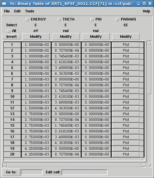
As all CCF constituents, the 2-D PSF CCF is a FITS file. Its content can be accessed through standard FTOOLS. The easiest way to visualise the content of a FITS file is through the FITS file viewer fv. The following image shows the content of the ELLBETA_PARAMS extension of the XRT1_XPSF_0011.CCF file (the XRT2* and XRT3* files have the same structure) as visualised by fv.

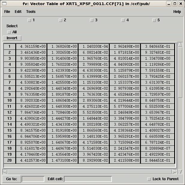Fig.1: fv view of the 2-D PSF CCF for XRT1. Left panel: the ELLBETA_PARAMS extension: Right panel: the content of the PARAMS column, once the function Expand under the Modify menu is activated. Legenda: ENERGY: the value E₀ of the energy grid node; THETA: the value θ₀ of the off-axis grid node; PHI: the value φ₀ of the azimuthal angle grid node (currently the 2-D PSF parametrisation is not dependent on the azimuthal angle): PARAMS: the parameters describing the King+Gaussian function envelope of the 2-D PSF: 1: the King function core radius r₀ (in arcseconds); 2: the King function power-law slope α; 3: the King function (also the Gaussian function) ellipticity ε; 4: the Gaussian Full Width Half Maximum (in arcseconds); 5: the ratio N between the Gaussian and the King function peak values

Users are recommended to read the fv manual to learn how to use it. However, its Graphical User Interface is rather straightforward, once a file is read with the command:

  fv XRT1_XPSF_0011.CCF &

FITS files can be also accessed through command-line driven FTOOLS. The following example shows how to display on the standard output the value of the power-law slope of the King function corresponding to the following input values: E₀=100 eV; θ₀=0.00261 radians; and φ₀=0:

  ftabpar fitsfile=XRT1_XPSF_0011.CCF+71 column=4 row=4 element=2
  pget ftabpar value

where 71 is the number of the ELLBETA_PARAMS extension in the CCF, and the interpretation of the other parameters in ftabpar is left as an exercise to the user. There are several different ways to achieve the same goal (using other FTOOLS such as fdump). The method shown above is - as far as the writer's experience can tell - the most robust to use in scripting.

If the user has no prior knowledge of the column/row/element to which a certain parameter for a certain term [E₀, θ₀, φ₀] correspond, the following loop (in C-shell syntax) may be used as template:

  #
  # Start a loop
  #
  @ i == 1
  #
  # Calculate the number of grid elements in the CCF
  #
  fkeypar fitsfile=/ccf/pub/XRT3_XPSF_0011.CCF+71 keyword=NAXIS2
  set nvalues = `pget fkeypar value`
  #
  # Loop on the grid points
  #
  loop:
  #
  # Determine the energy, off-axis and azimuthal angle corresponding
  # to each grid point
  #
  ftabpar fitsfile=/ccf/pub/XRT3_XPSF_0011.CCF+71 column=1 row=${i}
  set energy = `pget ftabpar value`
  ftabpar fitsfile=/ccf/pub/XRT3_XPSF_0011.CCF+71 column=2 row=${i}
  set theta = `pget ftabpar value`
  ftabpar fitsfile=/ccf/pub/XRT3_XPSF_0011.CCF+71 column=3 row=${i}
  set phi = `pget ftabpar value`
  #
  # Check if the grid point corresponds to the inputs
  # If so, read the corresponding profile power-law slope
  #
  if ("${energy} == ${e_0}" && "${phi} == ${f_0}" && "${theta} == ${t_0}") then
    ftabpar fitsfile=/ccf/pub/XRT3_XPSF_0011.CCF+71 column=4 row=4 element=2
    set slope = `pget ftabpar value`
    goto label_out
  endif
  #
  # End of the loop
  #
  @ i ++
  (if ${i} =< ${nvalues}) goto loop:
  label_out:

How to generate a PSF image for arbitrary [E₀, θ₀, φ₀]

calview
 

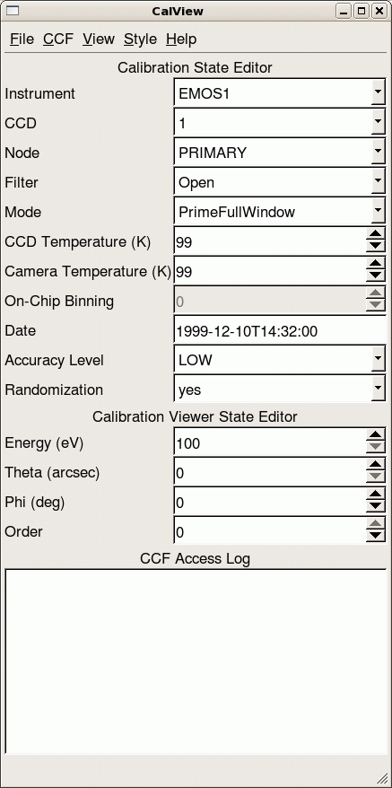
SAS includes a specific GUI tool to visualise CCF constituents: calview. Fig.2 shows the main calview window, which appears upon (C-shell syntax):

  setenv SAS_CCF ccf.cif
  calview &

Fig.2: the main calview window.
 

In Fig.3 we show two examples of the 2-D PSF generated through calview for different choices of the parameters E₀ and θ₀. Note that the input values in this example do not correspond to any of the predefined energy or off-axis angle grid nodes. calview interpolates between the closest points in the available grid. These images are produced using the option View->PSF from the GUI top menu and setting the Accuracy Level to ELLBETA.
 

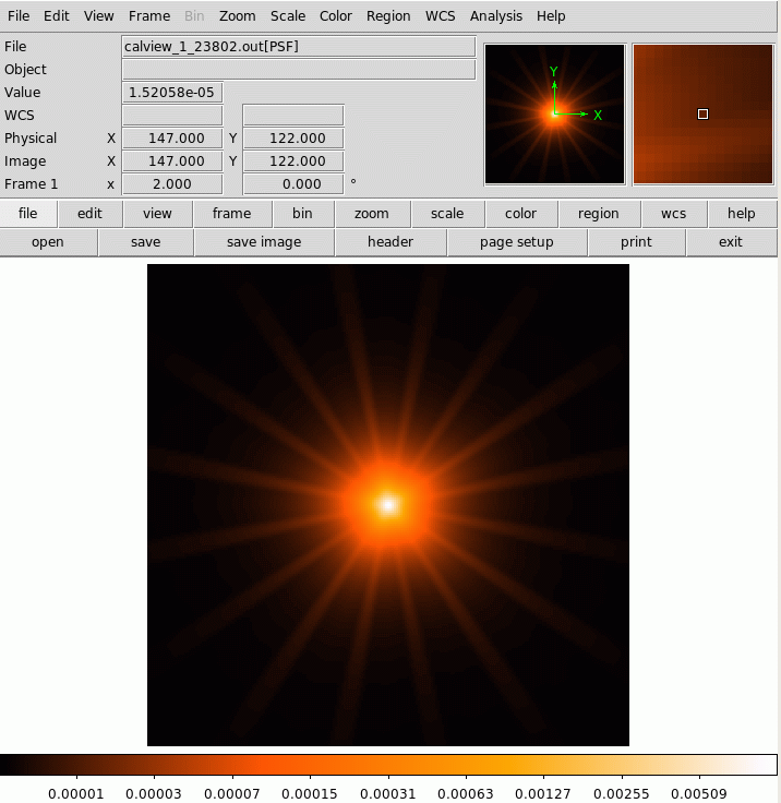
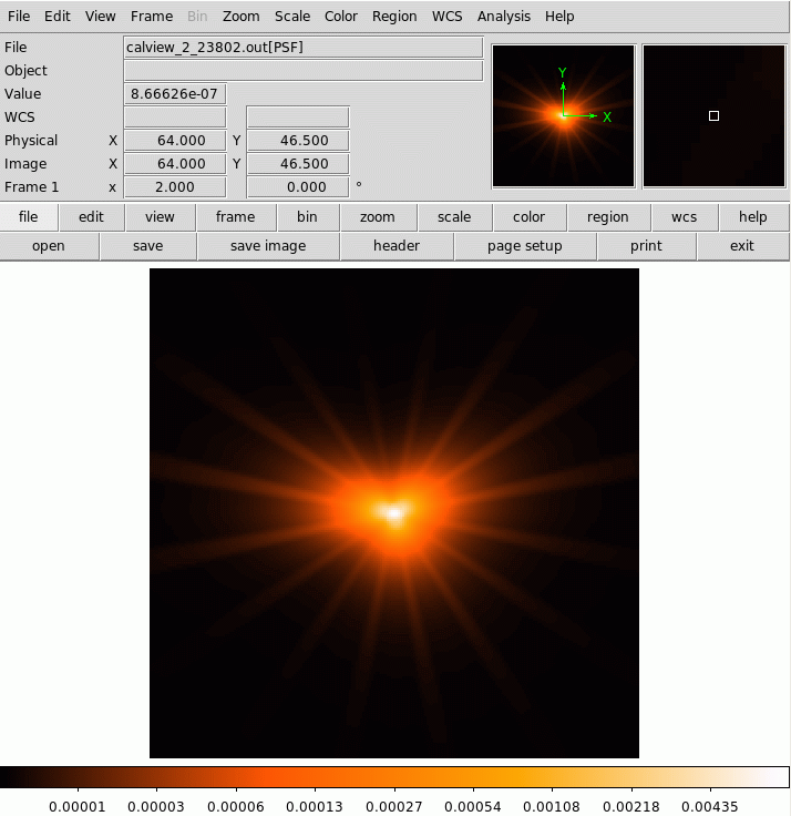
Fig.3: Examples of 2-D PSF generated by calview. Left panel: Instrument=EMOS1, Energy=500, Theta=120; Right panel: Instrument=EMOS2, Energy=1750, Theta=600. In both cases: Accuracy Level=ELLBETA.
 

The PSF files produced by calview are in FITS format, and can therefore be saved on the local disk, or manipulated with standard FTOOLS or ds9 (indeed calview automatically runs ds9 on them). However, these files are produced with a standard size, and cannot be customised to reproduce the exact PSF corresponding to the position of a specific source.
 

psfgen

The command-line task psfgen has been specifically designed with this purpose in mind, that is, to reproduce the exact PSF corresponding to the position of a specific source. Three examples are given below.

By running:

  psfgen energy=2500 coordtype=TEL x=600 y=0 xsize=1000 ysize=1000 \
     output=mos1_psf.img level=ELLBETA instrument='M1'

    the user generates a 1000x1000 pixels FITS image mos1_psf.img corresponding to the MOS1 2-D PSF for E₀=2500 eV and θ₀=10 arcminutes (=600 arcseconds). Pixels will have a fixed size of 1x1 arcsecond² for the ELLBETA or EXTENDED models (for other models, e.g. MEDIUM, the pixel size is 1.1x1.1 arcsecond² .

By running:

  psfgen image=mos1.img energy="100 2000 4500" weight="0.2 0.5 0.3" \
     output=mos1_psf.img level=ELLBETA coordtype=eqpos x=188.25 y=64.21

    the user generates a FITS image mos1_psf.img corresponding to the combination (with weights 0.2,0.5,0.3) of MOS1 PSFs of energy E₀=100, 2000, and 4500 eV at the celestial position (RA=188.25, DEC=64.21) within the MOS1 field-of-view imaged in mos1.img (this image having been created by xmmselect or evselect, and thus containing the correct DSS), with a default size of 199 x 199 pixels. The image of the PSF will be rotated by the position angle of the observation to have the correct orientation relative to the image mos1.img.

By running:

  psfgen instrument='M2' energy="100" coordtype=det x=10000 y=5000 \
     output=mos2_psf.img level=ELLBETA rotate=45 xsize=500 ysize=500

    the user generates a FITS image mos2_psf.img of the MOS2 PSF at 100eV of a source positioned at detector coordinate position (detx=10000, dety=5000), rotated by 45 degrees.

Users can find more information on the usage of psfgen in the on-line SAS documentation