COSMOS SAS Thread - esasimage - XMM-Newton

SAS Thread - esasimage - XMM-Newton

Creation of EPIC background subtracted, exposure corrected images

Introduction

This thread describes how to create EPIC background subtracted, exposure corrected images combining data from the three instruments.

Expected Outcome

The final outcome of this thread are adaptively smoothed images in two spectral bands. In the process of creating the images full field of view and outer annulus spectral products (source and model background spectra, RMFs, and ARFs) are produced as well as count, exposure, and background count images.

SAS Tasks to be Used

Prerequisites

SAS Startup Thread

Useful Links

This thread makes use of the image display software ds9 and the spectral fitting tool Xspec
This thread makes use of the ftool grppha
Cookbook for data analysis of extended sources using ESAS in SAS, on-line and PDF format - from NASA XMM-GOF.
ESAS warnings and watchouts page - from NASA XMM-GOF.

Caveats

Last Reviewed: 31 January 2025, for `SAS v22.0`

Last Updated: 25 May 2023

Procedure

This thread contains a step-by-step recipe to create EPIC background subtracted, exposure corrected images combining data from all three instruments.

Set up your SAS environment (following the SAS Startup Thread)
Create MOS and pn (including OOT processing) event files for your observation using emchain and epchain:

epchain
epchain withoutoftime=true
emchain

Note that epchain, by default, only does the first pn segment that it finds. Sometimes this is not all the pn data that there is. To determine how many pn data segments there are:

epchain exposure=99

Since there probably aren't 99 exposures, this will produce an error statement. It will also produce a list of pn segments:

-:-------------------------------------------------------------------- -:- ARGV = ! exposure=99 ! -:- Test: TIME RAWX RAWY DETX DETY X Y PHA PI FLAG PATTERN PAT_ID PAT_SEQ OFFSETX -:- Tested: TIME RAWX RAWY DETX DETY X Y PHA PI FLAG PATTERN PAT_ID PAT_SEQ OFFSETX -:- Test: double int16 int16 int16 int16 int32 int32 int16 int16 int32 int8 int16 int8 int16 -:- Tested: double int16 int16 int16 int16 int32 int32 int16 int16 int32 int8 int16 int8 int16 -:- EXPOSURE = 99 -:- 2 IMAGING exposures in ODF: -:- 1: 0100_0097820101_PNS005 IM -:- 2: 0100_0097820101_PNS013 IM ** -: error (exposure), exposure not found in /Users/kuntz/Data/xmm_nacho/0097820101/ODF directory. Check exposure index 99

You can process the nth segment with:

epchain exposure=n
Determine which MOS chips are in anomalous states using emanom:

emanom eventfile=mos1S003.fits emanom eventfile=mos2S004.fits

Note that emanom will indicate which CCDs are operating in an anomalous mode (B) or are not operating at all (O). These CCDs should be excluded in downstream processing. Whether or not a CCD is operating in an anomalous mode is not always clear (I or U). For those CCDs the user should consider the particular impact on their own science when deciding to include or exclude the chip for further processing.

1S003 M1 CCD: 2 Hard = 4.64406776 +/- 0.666529477 Status: G M1 CCD: 3 Hard = 5.26829290 +/- 0.897465289 Status: G M1 CCD: 4 Hard = 2.76271176 +/- 0.296809137 Status: I M1 CCD: 5 Hard = 1.59555554 +/- 0.135668769 Status: B M1 CCD: 6 Hard = 4.12727261 +/- 0.620288074 Status: G M1 CCD: 7 Hard = 4.73684216 +/- 0.690467894 Status: G Status: G is good at all energies : I is intermediate for E<1 keV : B is bad for E<1 keV : O is off, chip not in use : U is undetermined (low band counts <= 0)
2S004 M2 CCD: 2 Hard = 2.83838391 +/- 0.331735671 Status: G M2 CCD: 3 Hard = 3.95454550 +/- 0.544851601 Status: G M2 CCD: 4 Hard = 7.06976748 +/- 1.15185773 Status: G M2 CCD: 5 Hard = 3.69565225 +/- 0.434309751 Status: I M2 CCD: 6 Hard = 3.96721315 +/- 0.568374038 Status: G M2 CCD: 7 Hard = 3.88157892 +/- 0.499318421 Status: G Status: G is good at all energies : I is intermediate for E<1 keV : B is bad for E<1 keV : O is off, chip not in use : U is undetermined (low band counts <= 0)
Determine which time intervals are contaminated by soft proton flares and remove them to create cleaned event files for your observation with espfilt:

espfilt eventfile=mos1S003.fits method=histogram withsmoothing=yes smooth=51 rangescale=6.0 \ allowsigma=3.0
espfilt eventfile=mos2S004.fits method=histogram withsmoothing=yes smooth=51 rangescale=6.0 \ allowsigma=3.0
espfilt eventfile=pnS003.fits method=histogram withsmoothing=yes smooth=51 rangescale=15.0 \ allowsigma=3 withoot=Y ootfile=${PN}-oot.fits

espfilt filters an event file to remove periods with high soft proton flux. This routine is not fool-proof, and may fail if too much of the observation contains soft proton flares. Note that the call to espfilt for the pn is slightly different than the call for the MOS. It is essential to examine the diagnostic plots created by espfilt as they provide an indication of the quality of the data. These files have names like mos1S003-hist.qdp, mos2S004-hist.qdp, and pnS005-hist.qdp and can be plotted using the command, for example, qdp mos1S003-hist.qdp. Note that while much of the soft proton contamination is removed, there is likely to be some residual contamination left. Figure 1 shows the light-curve screening for the pn instrument.

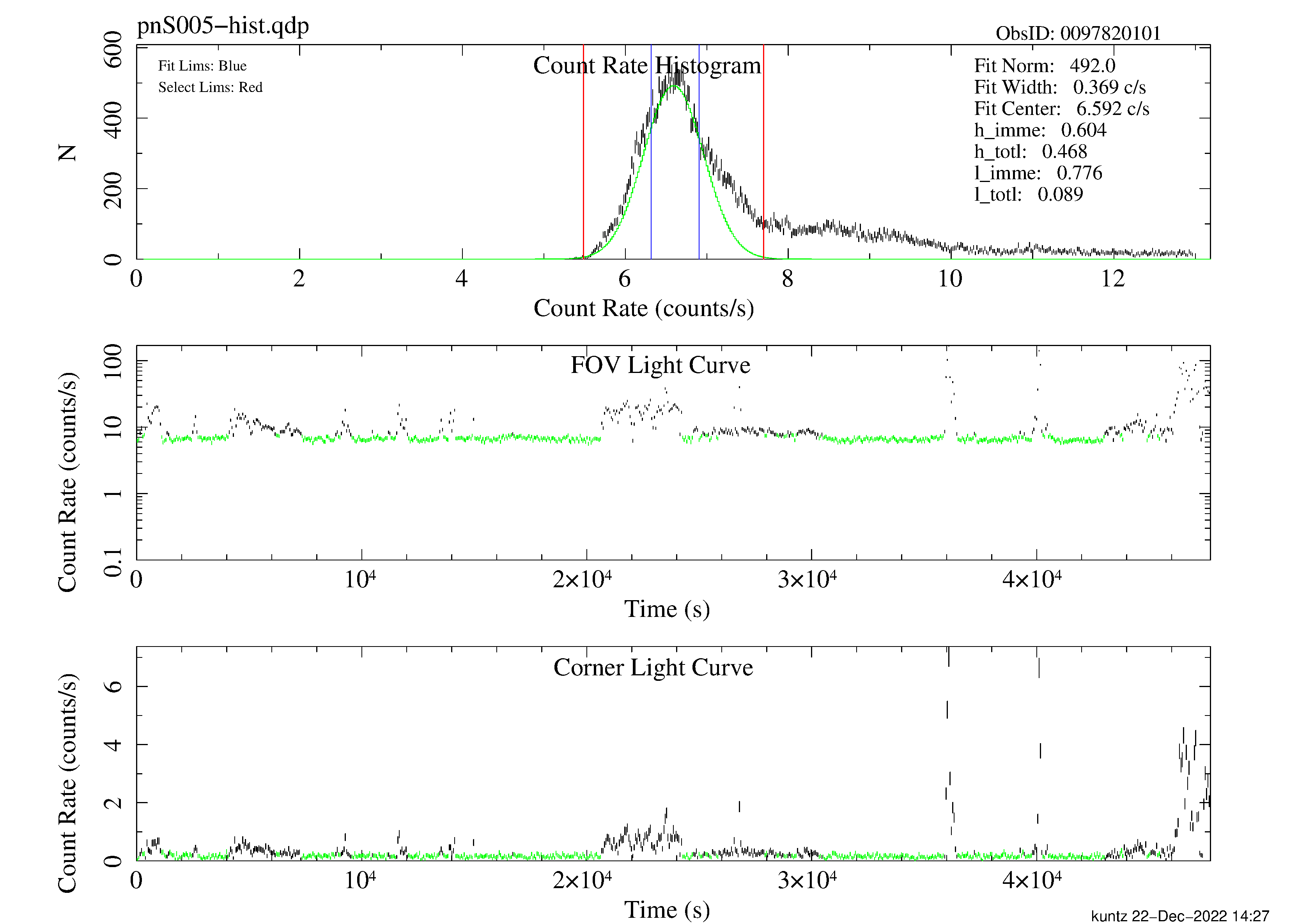
Figure 1: pn light curve for the Abell 1795 observation. Notice the residual variation of the nominally good data which indicates the possible existence of residual soft proton contamination. Note also that the pn detector is more sensitive to the soft protons than are the MOS detectors.
Run source detection and make point-source masks with cheese:

cheese mos1file=mos1S003-allevc.fits mos2file=mos2S004-allevc.fits pnfile=pnS003-allevc.fits \ pnootfile=pnS003-allevcoot.fits \ elowlist=400 ehighlist=1250 ratetotal=1.0 dist=50. keepinterfiles=false
Examine the MOS soft band images created by espfilt to confirm that the indicated CCDs are operating in an anomalous state, or that any other CCDs are not doing so, and verify that the point-source (cheese) masks look reasonable. Sometime artifacts may occur in regions of bright diffuse emission.

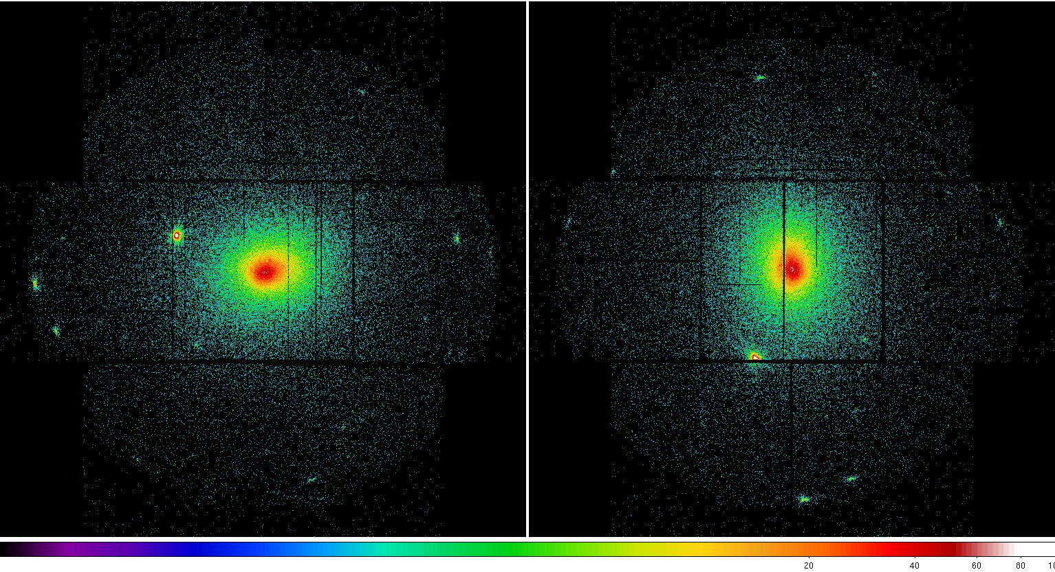
Figure 2: MOS1 (left) and MOS2 (right) images in the soft (0.2-1.0 keV) band. Note the excess counts in the upper left CCD in the MOS1 image most noticeable in the unexposed (to the sky) upper left corner. Displayed by the command: ds9 *soft* &

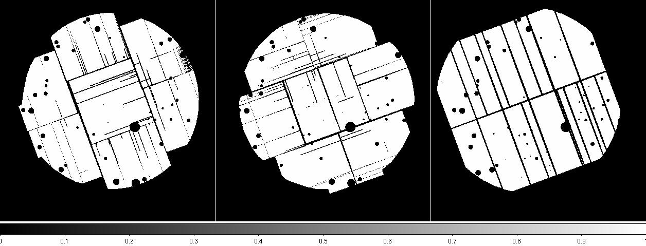
Figure 3: MOS1 (left), MOS2 (middle), and pn (right) cheese masks. Displayed by the command: ds9 *cheese* &
Use mosspectra and pnspectra to create the required intermediate spectra (for the entire region of interest as well as spectra from the individual CCDs), RMF and ARF files, and detector images for one band and three detectors. MOS CCDs affected by anomalous states should be deselected (this is done by the ccds parameter). For example, MOS1 CCD6 should be deselected if the observation took place after the meteorite damage. The region selection expression is input through the withregion and regionfile parameters. The region selection expression should be in detector coordinates. If withregion=false or the input file (regmos1.txt in this case) does not exist, the default is to process the entire FOV. The input energies are in eV.

mosspectra eventfile=mos1S003-allevc.fits withregion=yes regionfile=regmos1.txt \ pattern=12 withsrcrem=yes \    maskdet=mos1S003-bkgregtdet.fits masksky=mos1S003-bkgregtsky.fits elow=400 ehigh=1100 \ ccds="T T T F F T T"
mosspectra eventfile=mos2S004-allevc.fits withregion=yes regionfile=regmos2.txt \ pattern=12 withsrcrem=yes \    maskdet=mos2S004-bkgregtdet.fits masksky=mos2S004-bkgregtsky.fits elow=400 ehigh=1100 \ ccds="T T T T F T T"
pnspectra eventfile=pnS005-allevc.fits ootevtfile=pnS005-allevcoot.fits \ withregion=yes regionfile="regpn.txt" pattern=0 \    withsrcrem=yes maskdet=pnS005-bkgregtdet.fits masksky=pnS005-bkgregtsky.fits elow=400 ehigh=1100 \   quads="T T T T"

Note: successive runs of mosspectra or pnspectra may overwrite previously constructed files. From this point on, one can run the reduction for several different energy bands in parallel. However, changing regions would require starting over from this point. Thus, it is a good idea to keep note of what files exist before mosspectra so you can return to this point of the reduction if you need to.
Use mosback and pnback to create the quiescent particle background (QPB) spectra and images (in detector coordinates). mosback and pnback create QDP plot files which shows the source and model background spectra for the observation. Any discrepancies at higher energies probably indicate residual soft proton contamination, unless there are really hard and bright sources in the field. In the case of this observation the discrepancy at high energies is consistent with soft protons as a residual contamination was already expected from the light curve histogram. The QDP files have names like mos1S005-spec.qdp. The same CCD selection must be used here as were used in mosspectra and pnspectra.

mosback inspecfile=mos1S003-fovt.pi elow=400 ehigh=1100 ccds="T T T F F T T"
mosback inspecfile=mos2S004-fovt.pi elow=400 ehigh=1100 ccds="T T T T F T T"
pnback inspecfile=pnS005-fovt.pi inspecoot=pnS005-fovtoot.pi elow=400 ehigh=1100 quads="T T T T"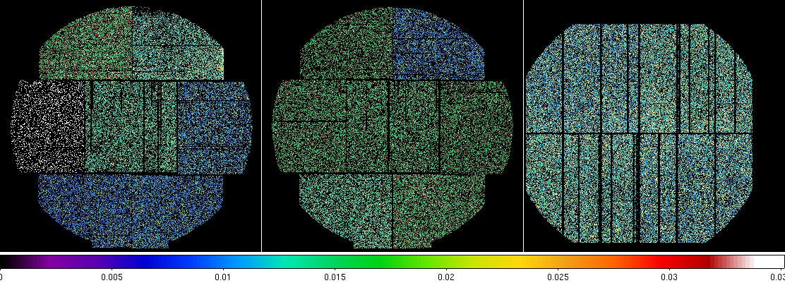

Figure 4: MOS1 (left), MOS2 (middle), and pn (right) model particle images in the soft (0.4-1.25 keV) band. The different colors for the different CCDs are an indication of the variations in their exposures. Displayed by the command: ds9 mos1S003-bkgimdet-400-1250.fits mos2S004-bkgimdet-400-1250.fits pnS005-bkgimdet-400-1250.fits &

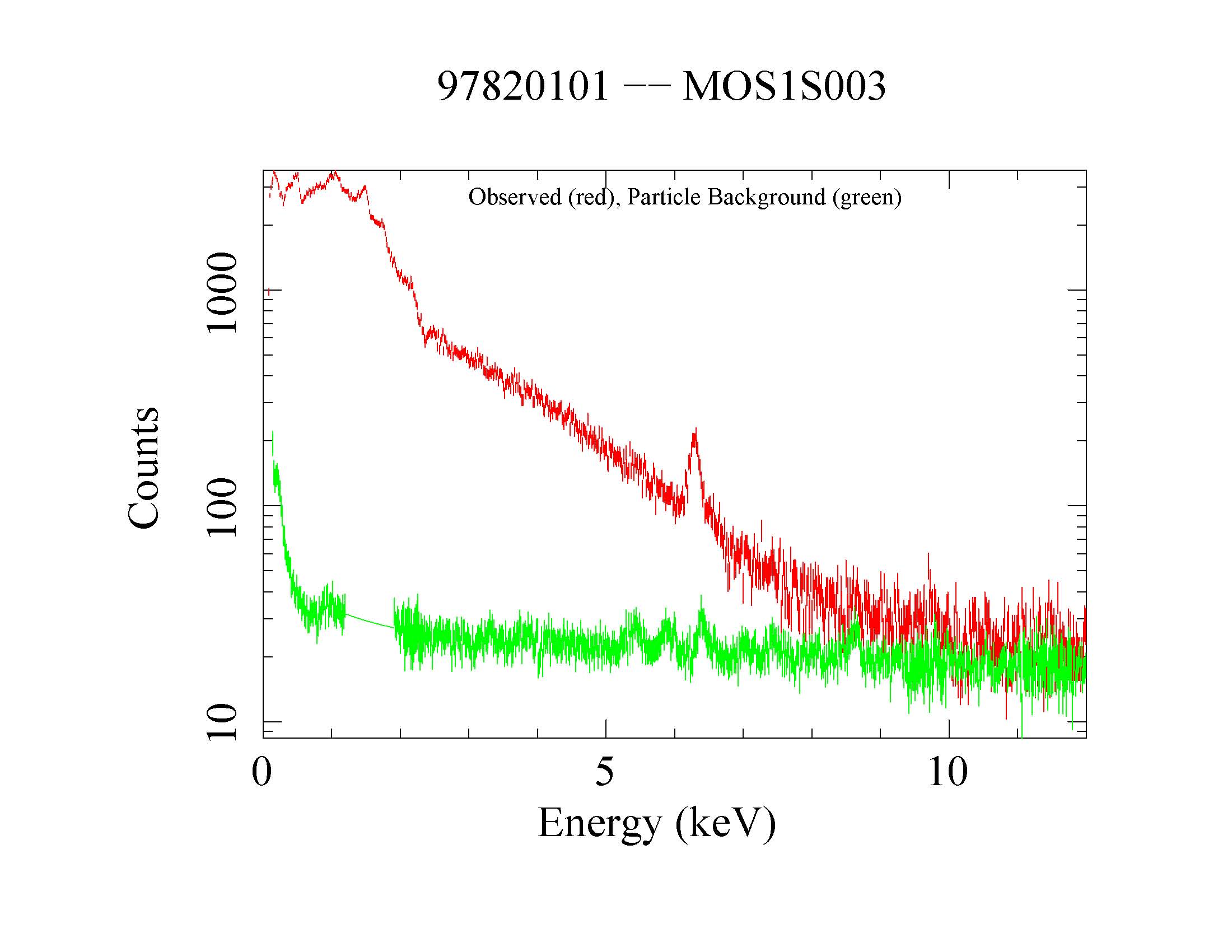
Figure 5: MOS1 source (red) and QPB (green) spectra. Displayed by the command: qdp mos1S003-bkgspec.qdp.

Note that the output images from mosback and pnback are in detector coordinates and need to be rotated into sky coordinates with rotdet2sky:

rotdet2sky intemplate=mos1S003-fovimsky-400-1250.fits inimage=mos1S003-bkgimdet-450-1250 \ outimage=mos1S003-bkgimsky-400-1250.fits withdetxy=false withskyxy=false rotdet2sky intemplate=mos2S004-fovimsky-400-1250.fits inimage=mos2S004-bkgimdet-450-1250 \ outimage=mos2S004-bkgimsky-400-1250.fits withdetxy=false withskyxy=false rotdet2sky intemplate=pnS005-fovimsky-400-1250.fits inimage=pnS005-bkgimdet-450-1250 \ outimage=pnS005-bkgimsky-400-1250.fits withdetxy=false withskyxy=false
Group the spectral data in preparation for spectral fitting:

grppha mos1S003-fovt.pi mos1S003-grp.pi \   'chkey BACKFILE mos1S003-bkg.pi & chkey RESPFILE mos1S003.rmf & \    chkey ANCRFILE mos1S003.arf & group min 1000 & exit'

grppha mos2S004-fovt.pi mos2S002-grp.pi \   'chkey BACKFILE mos2S004-bkg.pi & chkey RESPFILE mos2S004.rmf & \    chkey ANCRFILE mos2S004.arf & group min 1000 & exit'

grppha pnS005-fovtootsub.pi pnS005-grp.pi \   'chkey BACKFILE pnS005-bkg.pi & chkey RESPFILE pn0.rmf & \    chkey ANCRFILE pnS005.arf & group min 100 & exit'
Fit the spectral data to determine the soft proton contamination parameters. (You may be able to determine the SWCX parameters as well, though this is more problematic!) This fitting is aided by getting the ROSAT All-Sky Survey (RASS) spectrum of the region from the HEASARC X-ray background tool along with the appropriate spectral response matrix (rass.pi and pspcc.rsp in this Xspec XCM file). The region selected for the RASS spectrum should be typical of the nominal background in the direction of your source. For example, the spectrum in an annulus surrounding a cluster of galaxies. The fitted model is fairly complex with components representing the cosmic diffuse X-ray background (an unabsorbed thermal component about 0.1 keV, and absorbed thermal component about 0.25 keV, and the extragalactic power law with a spectral index of 1.46), a component representing your source, Gaussian lines at 1.496 keV and 1.75 keV representing the Al Kalpha and Si Kalpha lines in the MOS, lines at 1.496 keV and near 8 keV representing the Al Kalpha and Cu lines in the pn, possible solar wind charge exchange (SWCX) lines at 0.56 and 0.65 keV, and a broken power law representing the residual soft proton contamination (MOS and pn only, fitted with a diagonal matrix, mos1-diag.rsp.gz, mos2-diag.rsp.gz, and pn-diag.rsp.gz). The cosmic background parameters should be linked for all spectra, your source spectrum parameters should be linked for all spectra but the normalization should be fixed at 0 for the RASS data. The SWCX parameters should be linked for all spectra but the normalization should be fixed at 0 for the RASS data. The parameters for the soft proton background should be independent except that the power law index for the two MOS detectors can be linked. The non-detector components of the fit should be scaled by the solid angle in square arc minutes (the RASS spectrum is already in these units). The solid angle in 0.05 arcsec by 0.05 arcsec pixels is in the BACKSCAL parameter in the header of the spectra. Alternatively protonscale can be used to find the solid angle for the region to include in the spectral fitting.

protonscale mode=1 maskfile=mos1S003-fovimspdet.fits specfile=mos1S003-fovt.pi
protonscale mode=1 maskfile=mos2S004-fovimspdet.fits specfile=mos2S004-fovt.pi
protonscale mode=1 maskfile=pnS005-fovimspdet.fits specfile=pnS005-fovt.pi

The result of the fitting process is shown in Figure 6.

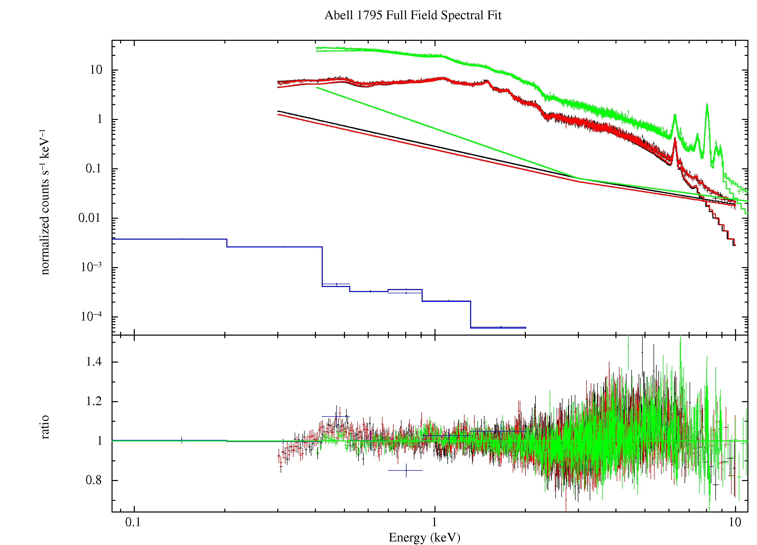
Figure 6: Best fit of the Abell 1795 data from the full FOV. The green data and model curves are from the pn, the black and red data and model curves are from the MOS1 and MOS2, respectively, and the blue model and curve are from the RASS. The single kinked but otherwise straight line model curves for the MOS and pn are the soft proton contributions (broken power law).
Create an image of the soft proton contamination using proton. This routine uses the fitted soft proton parameters to create images of the soft proton contamination in detector coordinates. Note that this routine uses the normalization for the entire field of view:

proton imagefile=mos1S004-fovimdet-400-1250.fits specfile=mos1S004-fovt.pi ccds="T T T F F T T" \ elow=400 ehigh=1250 speccontrol=2 bbreak=3.0 bindl=1.35623 bindh=1.00895 bnorm=0.284155 proton imagefile=mos2S005-fovimdet-400-1250.fits specfile=mos2S005-fovt.pi ccds="T T T T F T T" \ elow=400 ehigh=1250 speccontrol=2 bbreak=3.0 bindl=1.35623 bindh=1.00895 bnorm=0.243166 proton imagefile=pnS003-fovimdet-400-1250.fits specfile=pnS003-fovt.pi ccds="T T T T" \ elow=400 ehigh=1250 speccontrol=2 bbreak=3.0 bindl=2.12156 bindh=0.813229 bnorm=0.654548

Note that proton creates an image in detector coordinates which must be rotated into sky coordinates:

rotdet2sky intemplate=mos1S003-fovimsky-400-1250.fits inimage=mos1S003-protimdet-450-1250 \ outimage=mos1S003-protimsky-400-1250.fits withdetxy=false withskyxy=false rotdet2sky intemplate=mos2S004-fovimsky-400-1250.fits inimage=mos2S004-protimdet-450-1250 \ outimage=mos2S004-protimsky-400-1250.fits withdetxy=false withskyxy=false rotdet2sky intemplate=pnS005-fovimsky-400-1250.fits inimage=pnS005-protimdet-450-1250 \ outimage=pnS005-protimsky-400-1250.fits withdetxy=false withskyxy=false
If we had fitted parameters for the solar wind charge exchange (swcx), swcx uses the fitted swcx parameters to create images of the swcx contamination in detector coordinates. Note that this routine uses the normalization per square arcminute. The analysis of this observation did not require swcx. But if it had, the commands would look like:

swcx imagefile=mos1S004-fovimdet-400-1250.fits specfile=mos1S004-fovt.pi ccds="T T T F F T T" \ elow=400 ehigh=1250 lines="OVII OVIII" gnorms="1.69938e-7 1.75262e-8" swcx imagefile=mos2S005-fovimdet-400-1250.fits specfile=mos2S005-fovt.pi ccds="T T T T F T T" \ elow=400 ehigh=1250 lines="OVII OVIII" gnorms="1.69938e-7 1.75262e-8" swcx imagefile=pnS003-fovimdet-400-1250.fits specfile=pnS003-fovt.pi ccds="T T T T" \ elow=400 ehigh=1250 lines="OVII OVIII" gnorms="1.69938e-7 1.75262e-8"

Note that swcx creates an image in detector coordinates which must be rotated into sky coordinates:

rotdet2sky intemplate=mos1S003-fovimsky-400-1250.fits inimage=mos1S003-swcximdet-450-1250 \ outimage=mos1S003-swcximsky-400-1250.fits withdetxy=false withskyxy=false rotdet2sky intemplate=mos2S004-fovimsky-400-1250.fits inimage=mos2S004-swcximdet-450-1250 \ outimage=mos2S004-swcximsky-400-1250.fits withdetxy=false withskyxy=false rotdet2sky intemplate=pnS005-fovimsky-400-1250.fits inimage=pnS005-swcximdet-450-1250 \ outimage=pnS005-swcximsky-400-1250.fits withdetxy=false withskyxy=false
At this point all of the components for all three instruments are ready to create an image. Figure 7 displays the components for MOS1.

Figure 7: MOS1 image components with the count image (upper left), exposure image (upper right), QPB image (lower left), and soft proton image lower right.
The routine combimage combines the MOS1, MOS2, and pn images, as well as images from multiple exposures. Since the spectra and images were created with point sources removed combimage must be run using the cheese masking.

combimage prefixlist='1S004 2S005 S003' withpartbkg=true withspbkg=true \ withswcxbkg=false \ pwithcheese=true cheesetype=t elowlist=400 ehighlist=1250

Had there been a SWCX image, then withswcxbkg=true would have been used.

Figure 8 shows the merged component images.

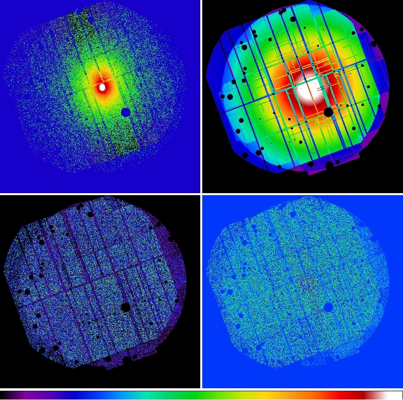
Figure 8: Merged image components with the count image (upper left), exposure image (upper right), QPB image (lower left), and soft proton image lower right. The negative counts in the count image are an artifact of the pn OOT correction.
The routine binadapt bins, adaptively smooths, or bins and smooths the images.

binadapt prefix=comb elow=400 ehigh=1250 withpartbkg=true withswcxbkg=false \ withspbkg=true withmask=false withbinning=true binfactor=4 withsmoothing=false binadapt prefix=comb elow=400 ehigh=1250 withpartbkg=true withswcxbkg=false \ withspbkg=true withmask=false withbinning=false binfactor=1 withsmoothing=true \ smoothcounts=50 binadapt prefix=comb elow=400 ehigh=1250 withpartbkg=true withswcxbkg=false \ withspbkg=true withmask=false withbinning=true binfactor=4 withsmoothing=true \ smoothcounts=50

Figure 9 shows the final adaptively smoothed, background subtracted, and exposure corrected images.

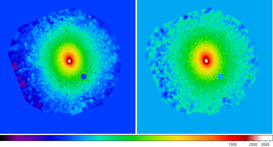
Figure 9: Abell 1795 adaptively smoothed, background subtracted, and exposure corrected images in the 0.4-1.25 keV and 2.0-7.2 keV bands.

The above sequence would work well for a "blank sky" observation. However, one might note that our fitting for the SP contamination could have been better for the observation used here. The bright cluster emission at the center of the field of view can overpower the SP signal. A better fit should be obtained if the extraction region is restricted to the outer annulus. The normalization from this fit will, of course, be reduced since it is made from a smaller region. Thus, the normalization will need to be scaled from the fitted region to full field of view. AT THIS POINT YOU NEED TO MOVE EVERYTHING MADE after MOSSPECTRA and PNSPECTRA INTO A BACKUP DIRECTORY.
Create the regmos1-ann.txt, regmos2-ann.txt, and regpn-ann.txt selection expressions. Note that the regions should cover the same part of the sky. Since the pn optical axis is offset from the center of the detector so on-axis sources will not fall in the chip gap, the annulus is smaller than the active areas.

regm1-ann.txt: &&((DETX,DETY) IN circle(134,-219,14200))&&!((DETX,DETY) IN circle(134,-219,10600)) regm2-ann.txt: &&((DETX,DETY) IN circle(6,-93,14200))&&!((DETX,DETY) IN circle(6,-93,10600)) regpn-ann.txt: &&((DETX,DETY) IN circle(59,-10,14200))&&!((DETX,DETY) IN circle(59,-10,10600))

Run mos-spectra, pn-spectra, mos_back, and, pn_back to do the spectral extraction and prepare for the background modeling. You don't actually need the images that are produced, but they can be useful to diagnose problems.

mosspectra eventfile=mos1S003-allevc.fits withregion=yes regionfile=regmos1-ann.txt \ pattern=12 withsrcrem=yes \ maskdet=mos1S003-bkgregtdet.fits masksky=mos1S003-bkgregtsky.fits \ elow=400 ehigh=1250 ccds="T T T F F T T" mosspectra eventfile=mos2S004-allevc.fits withregion=yes regionfile=regmos2-ann.txt \ pattern=12 withsrcrem=yes \ maskdet=mos2S004-bkgregtdet.fits masksky=mos2S004-bkgregtsky.fits \ elow=400 ehigh=1250 ccds="T T T T F T T" pnspectra eventfile=pnS005-allevc.fits ootevtfile=pnS005-allevcoot.fits \ withregion=yes regionfile="regpn-ann.txt" pattern=0 \ withsrcrem=yes maskdet=pnS005-bkgregtdet.fits masksky=pnS005-bkgregtsky.fits \ elow=400 ehigh=1250 quads="T T T T"

mosback inspecfile=mos1S003-fovt.pi elow=400 ehigh=1250 ccds="T T T F F T T" mosback inspecfile=mos2S004-fovt.pi elow=400 ehigh=1250 ccds="T T T T F T T" pnback inspecfile=pnS005-fovt.pi inspecoot=pnS005-fovtoot.pi elow=400 ehigh=1250 quads="T T T T"
Group the spectral data in preparation for spectral fitting:

grppha mos1S003-fovt.pi mos1S003-grp.pi \ 'chkey BACKFILE mos1S003-bkg.pi & chkey RESPFILE mos1S003.rmf & \ chkey ANCRFILE mos1S003.arf & group min 1000 & exit' grppha mos2S004-fovt.pi mos2S002-grp.pi \ 'chkey BACKFILE mos2S004-bkg.pi & chkey RESPFILE mos2S004.rmf & \ chkey ANCRFILE mos2S004.arf & group min 1000 & exit' grppha pnS005-fovtootsub.pi pnS005-grp.pi \ 'chkey BACKFILE pnS005-bkg.pi & chkey RESPFILE pn0.rmf & \ chkey ANCRFILE pnS005.arf & group min 100 & exit'
Determine the solid angle and fit the data using protonscale:

protonscale mode=1 maskfile=mos1S003-fovimspdet.fits specfile=mos1S003-fovt.pi protonscale mode=1 maskfile=mos2S004-fovimspdet.fits specfile=mos2S004-fovt.pi protonscale mode=1 maskfile=pnS005-fovimspdet.fits specfile=pnS005-fovt.pi

Fit the spectral data to determine the soft proton contamination parameters (Xspec XCM file). Note that the fitting process is complicated with a strong likelihood of local minima. The Al, Si, and Cu fluorescent background lines in particular should start frozen until a reasonably good fit is achieved and then thawed. After a new, and probably a significantly better fit is achieved they can be frozen again to reduce the number of free parameters and again improve the fit.

The result of the annular fitting process is shown if Figure 10. The cluster emission is now relatively minor allowing for a much improved fit to the various background components.

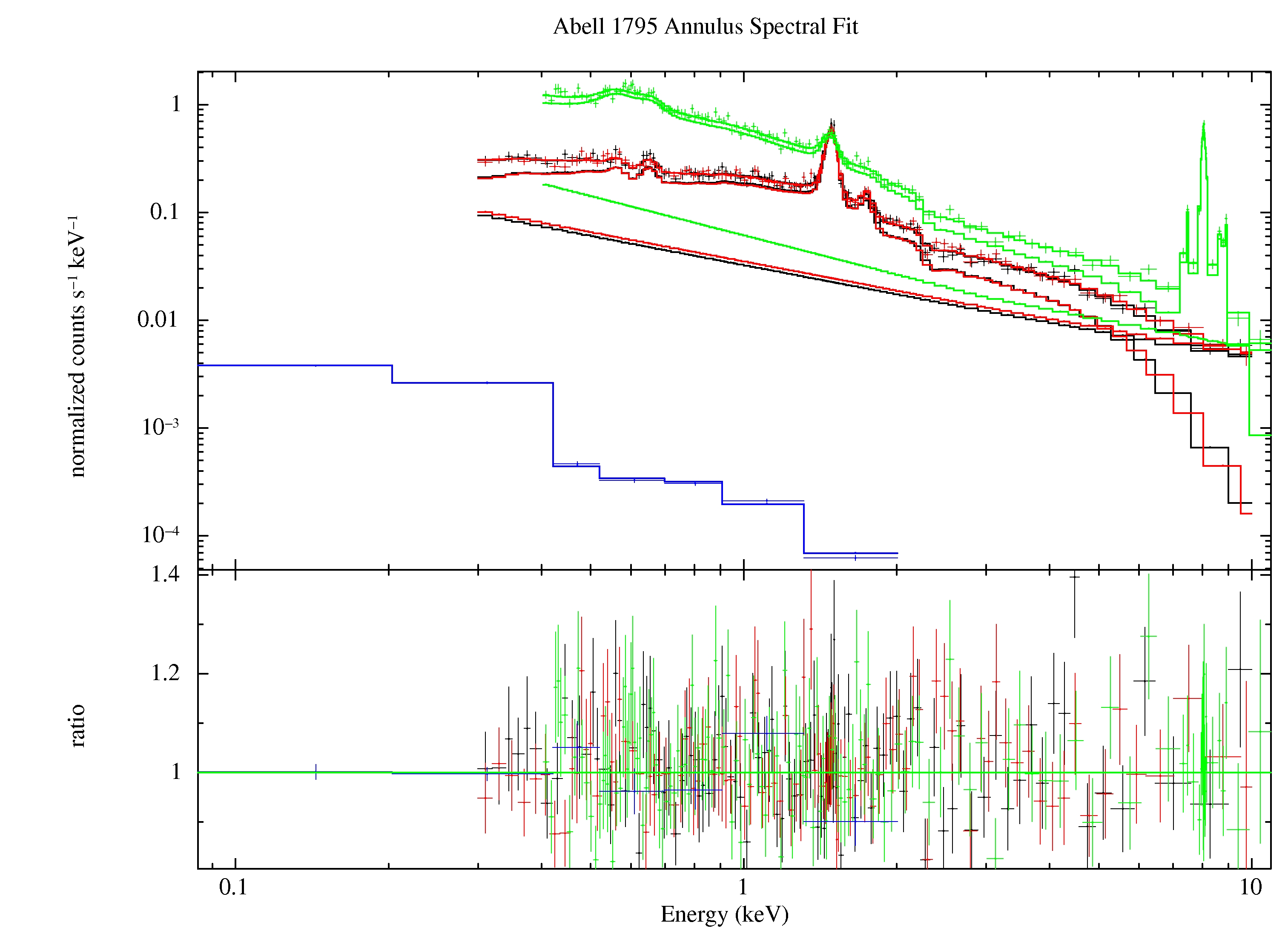
Figure 10: Best fit of the Abell 1795 data from the outer annulus. The green data and model curves are from the pn, the black and red data and model curves are from the MOS1 and MOS2, respectively, and the blue model and curve are from the RASS. The straight line model curves for the MOS and pn are the soft proton contribution.
Scale the fitted SP results for the limited region to the whole FOV with sppartial:

sppartial fullimage=mos1S004-fovimspdet.fits fullspec=mos1S004-fovt.pi \ regimage=mos1S004-fovimspdet-ann.fits \ regspec=mos1S004-fovt-ann.pi regnorm=3.23086E-02 sppartial fullimage=mos2S005-fovimspdet.fits fullspec=mos2S005-fovt.pi \ regimage=mos2S005-fovimspdet-ann.fits \ regspec=mos2005-fovt-ann.pi regnorm=3.49869E-02 sppartial fullimage=pnS003-fovimspdet.fits fullspec=pnS003-fovt.pi \ regimage=pnS003-fovimspdet-ann.fits \ regspec=pnS003-fovt-ann.pi regnorm=6.13648E-02
Using the output from sppartial, use proton to create images of the soft proton contamination in detector coordinates. Use the fitted power law index from the annular fit:

proton imagefile=mos1S004-fovimdet-400-1250.fits specfile=mos1S004-fovt.pi \ ccds="T T T F F T T" elow=400 ehigh=1250 speccontrol=2 bbreak=3.0 \ bindl=0.894423 bindh=0.833232 bnorm=0.1083109 proton imagefile=mos2S005-fovimdet-400-1250.fits specfile=mos2S005-fovt.pi \ ccds="T T T T F T T" elow=400 ehigh=1250 speccontrol=2 bbreak=3.0 \ bindl=0.894423 bindh=0.833232 bnorm=0.1174388 proton imagefile=pnS003-fovimdet-400-1250.fits specfile=pnS003-fovt.pi \ ccds="T T T T" elow=400 ehigh=1250 speccontrol=2 bbreak=3.0 \ bindl=1.20804 bindh=0.906014 bnorm=0.2093526

Use rot-im-det-sky again to rotate the detector coordinate soft proton background images into sky coordinates.

rotdet2sky intemplate=mos1S003-fovimsky-400-1250.fits \ inimage=mos1S003-protimdet-450-1250 \ outimage=mos1S004-protimsky-400-1250.fits withdetxy=false withskyxy=false rotdet2sky intemplate=mos2S004-fovimsky-400-1250.fits \ inimage=mos2S004-protimdet-450-1250 \ outimage=mos2S004-protimsky-400-1250.fits withdetxy=false withskyxy=false rotdet2sky intemplate=pnS005-fovimsky-400-1250.fits \ inimage=pnS005-protimdet-450-1250 \ outimage=pnS005-protimsky-400-1250.fits withdetxy=false withskyxy=false
combimage combines the MOS1, MOS2, and pn images, as well as images from multiple exposures. Since the spectra and images were created with point sources removed comb must be run using the cheese masking.

combimage prefixlist='1S004 2S005 S003' withpartbkg=true withspbkg=true \ withswcxbkg=false withcheese=true cheesetype=t elowlist=400 ehighlist=1250
Adaptively smooth the images.

binadapt prefix=comb elow=400 ehigh=1250 withpartbkg=true withswcxbkg=false \ withspbkg=true withmask=false withbinning=true binfactor=4 withsmoothing=false

Figure 11 shows the final adaptively smoothed, background subtracted, and exposure corrected images, this time with the better parametrization of the background components allowed by using the outer annulus. The effect is most clearly shown in the 0.4-1.25 keV band where the background is no longer over-subtracted.

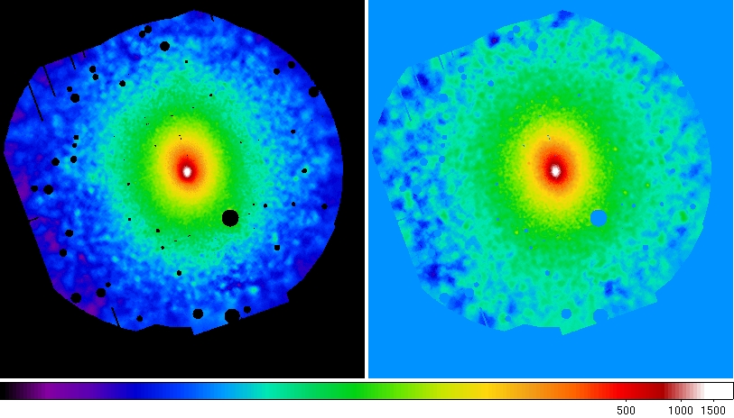
Figure 11: Abell 1795 adaptively smoothed, background subtracted, and exposure corrected images in the 0.4-1.25 keV and 2.0-7.2 keV bands.