
 Sign in
SAS Thread - images - XMM-Newton
How to Generate vignetting-corrected background-subtracted EPIC images
|
Introduction This threads deals with the creation of EPIC vignetting-corrected background-subtracted images. The method described in this thread can only be applied to images from EPIC-pn Full Frame and Extended Full Frame mode and EPIC-MOS Full Frame mode exposures. This thread briefly explains how to create such images for a particularscience observation. For this purpose, the XMM-Newton observation with id 0555630101 will be used throughout the thread. The observation corresponds to the extended source SN 1006-1, which is more suitable to illustrate image creation. Expected Outcome The expected outcome of this thread is a set of background-subtracted and vignetting-corrected EPIC science exposure images for different energy bands. For each energy band, an image of the science exposure, corresponding scaled out-of-time (OOT) (EPIC-pn only) and scaled Filter Wheel Closed (FWC) images, and a vignetting corrected exposure map and mask are created. This set of images is used to create the final background-subtracted and vignetting-corrected science exposure images for each energy band. SAS Tasks to be Used Prerequisites
Useful Links
Last Reviewed: 31 January 2025, for SAS v22.0Last Updated: 30 October 2020 |
Procedure
- Set up your SAS environment (see Prerequisites for this thread at the top of the page).
- Create standard EPIC event files for your science observation (see Prerequisites for this thread at the top of the page). The name of the event files for the example obsid used are:
1594_0555630101_EPN_S003_ImagingEvts.ds ; in Extended Full Frame mode
1594_0555630101_EMOS1_S001_ImagingEvts.ds ; in Full Frame mode
1594_0555630101_EMOS2_S002_ImagingEvts.ds ; in Full Frame mode
Additionaly, for EPIC-pn, an Out-of-Time event file has to be created first. Run epproc with the option withoutoftime set to yes. It is best to run first epproc with this option to produce the out-of-time event file and then produce the standard file to avoid overwritting files:
epproc withoutoftime=yes
For the example obsid, 0555630101, rename the produced file to indicate that it corresponds to Out-of-Time events:
1594_0555630101_EPN_S003_ImagingEvts.ds
to:
1594_0555630101_EPN_S003_OoT_ImagingEvts.ds
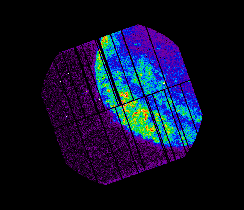
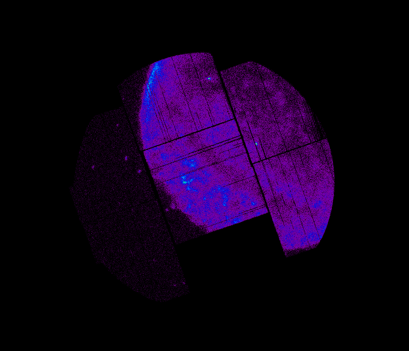
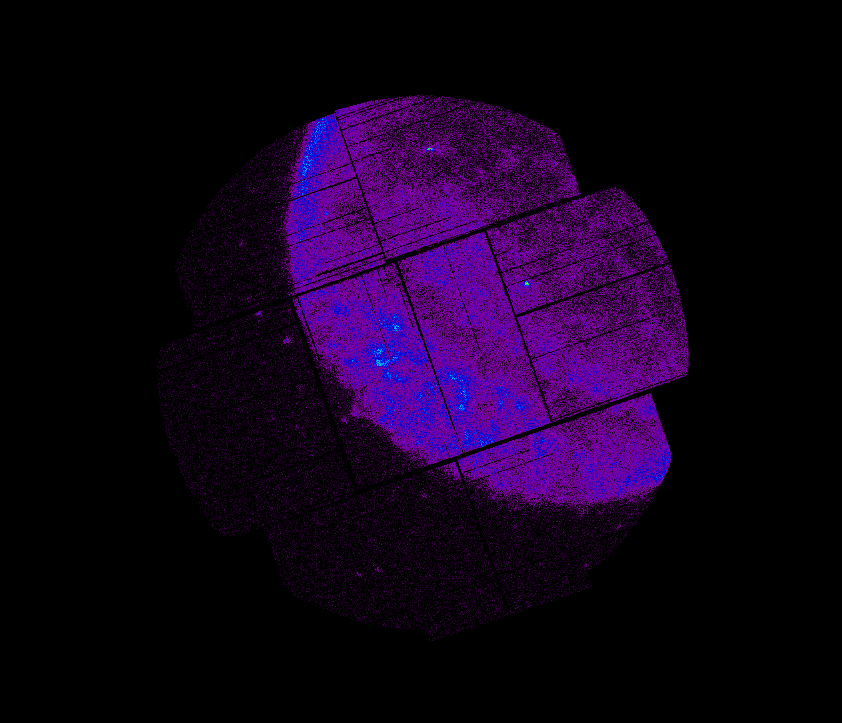
Fig.1: Individual raw EPIC (from left to right; pn, MOS1 and MOS2) images in the 0.2-12 keV energy range. The plotting scale of the three images is the same, so images can be visually compared directly. - If necessary, create Good Time Intervals (GTI) files defining time intervals clean of flaring particle background for your observation (see Prerequisites for this thread at the top of the page). The filtering procedure will result in a file with the definition of the GTI. It is not necessary to create a clean event file using these GTI files as the task eimageget will take care of it (see Caveats section at the bottom of this page). Let the name of the GTI files be:
pn_gti.fits
m1_gti.fits
m2_gti.fits
These files can be used as input for eimageget through the task parameter gtifile. Notice that this GTI selection will not be applied to the Filter Wheel Close event file produced by eimageget as it is not needed.
- Download the corresponding Filter Wheel Closed files from the repository and place them in the working directory together with the event files just created. In this case the needed files are:
pn_closed_EFF_2019_v1.fits.gz ; for Extended Full Frame mode
mos1_closed_FF_2019_v1.fits.gz ; for Full Frame mode
mos2_closed_FF_2019_v1.fits.gz ; for Full Frame mode
where 2019 in the file name in this example indicates the year. Download the latest files available.
- In its simplest form, run the SAS task eimageget over each one of the EPIC event files.
eimageget evtfile=1594_0555630101_EPN_S003_ImagingEvts.ds \
ootfile=1594_0555630101_EPN_S003_OoT_ImagingEvts.ds \
fwcfile=pn_closed_EFF_2019_v1.fits.gz \
gtifile=pn_gti.fits \
attfile=1594_0555630101_AttHk.ds
eimageget evtfile=1594_0555630101_EMOS1_S001_ImagingEvts.ds \
fwcfile=mos1_closed_FF_2019_v1.fits.gz \
gtifile=m1_gti.fits \
attfile=1594_0555630101_AttHk.ds
eimageget evtfile=1594_0555630101_EMOS2_S002_ImagingEvts.ds \
fwcfile=mos2_closed_FF_2019_v1.fits.gz \
gtifile=m2_gti.fits \
attfile=1594_0555630101_AttHk.ds
Notice that the Out-of-Time event file is only used in the call to eimageget for the case of EPIC-pn. These three calls will generate the following set of files:
P0555630101[PNS003,M1S001,M2S002]_ima_[0-4].fits ; science exposure images
P0555630101PNS003_ima_[0-4]oot.fits ; Out-of-Time exposure images (only for PN)
P0555630101[PNS003,M1S001,M2S002]_ima_[0-4]fwc.fits ; Filter Wheel Close exposure images
P0555630101[PNS003,M1S001,M2S002]_ima_[0-4]exp.fits ; Exposure maps
P0555630101[PNS003,M1S001,M2S002]_ima_mask.fits ; A single mask valid for all energy bandsWhere [0-4] indicates a different energy range, by default:
0: 0.2-0.5 keV
1: 0.5-1.0 keV
2: 1.0-2.0 keV
3: 2.0-4.5 keV
4: 4.5-12.0 keV
A set of different energy ranges can be specified by using the task parameters pimin and pimax in the call to eimageget.
Fig.2 shows the different images produced by eimageget for the case of EPIC-pn (the mask file is not shown). A similar result is obtained for EPIC-MOS1 and EPIC-MOS2.
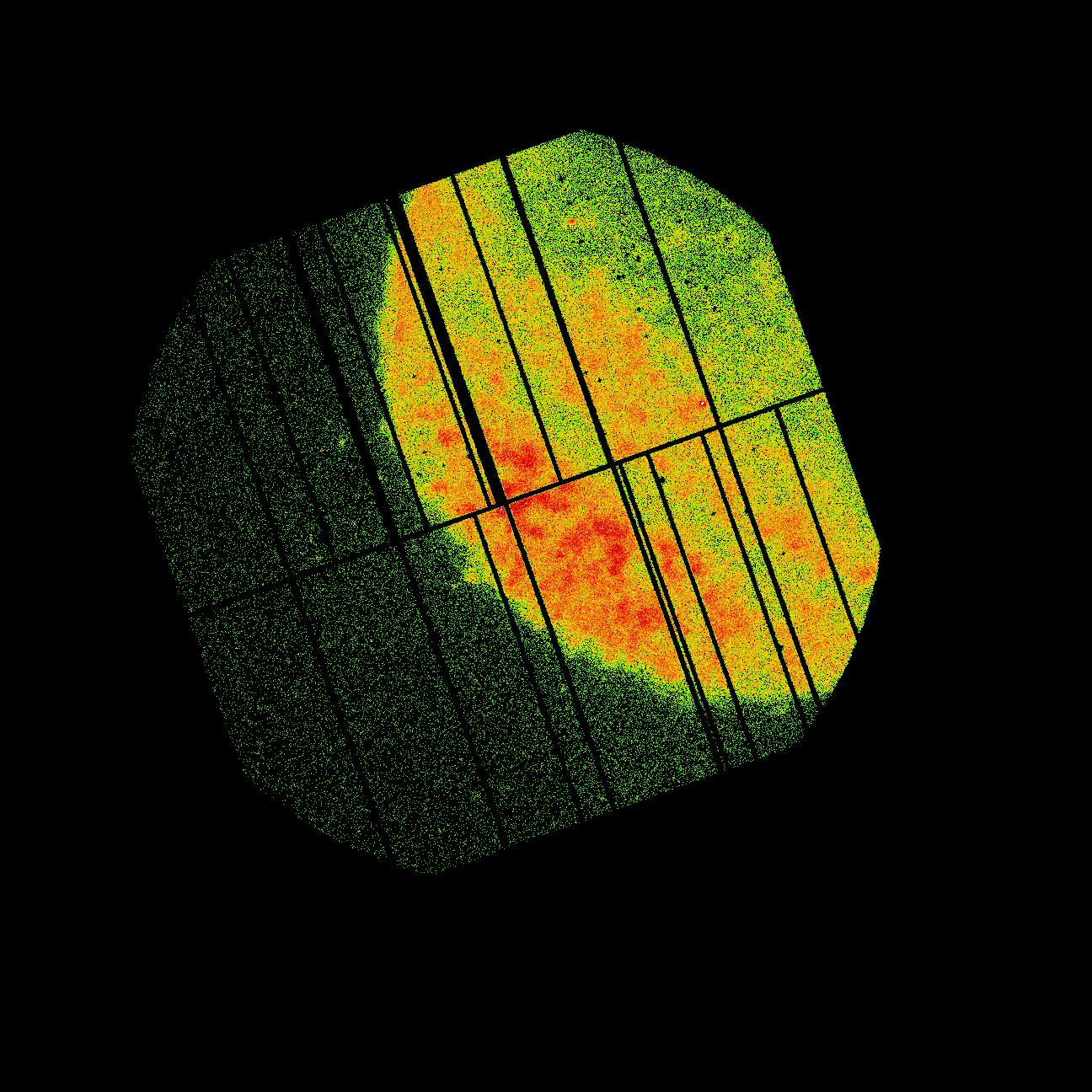
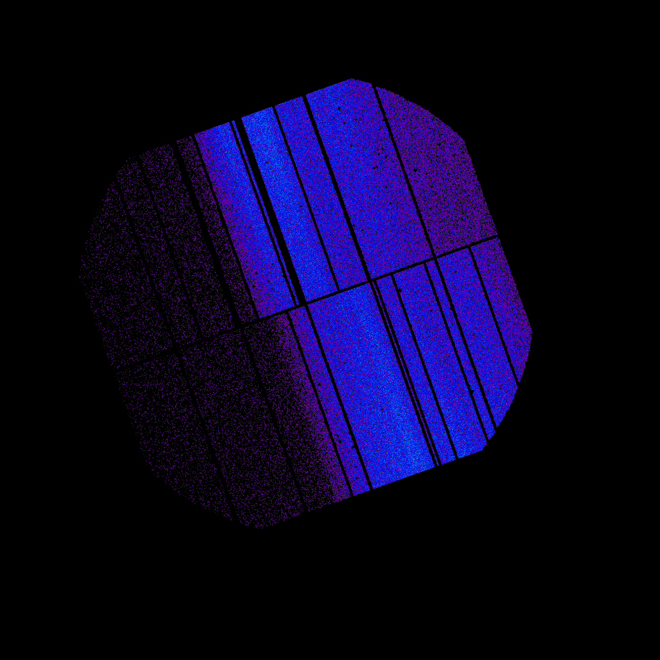
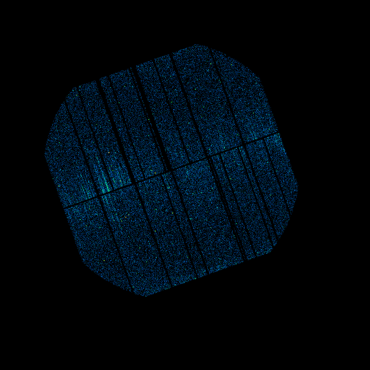
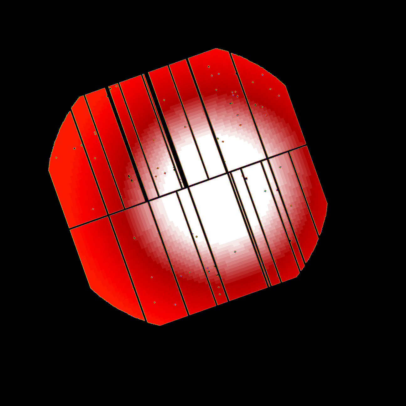
Fig.2: Result of applying eimageget to the EPIC-pn science exposure. Images correspond to the lowest energy range, 0.2-0.5 keV. From top lef to bottom right; science exposure image, scaled Out-of-Time exposure image, scaled Filter Wheel Close exposure image, and exposure map.
The plotting scale of the first three images is the same, so images can be visually compared directly. - The scaled Out-of-Time and Filter Wheel Close images can be subtracted directly from the corresponding exposure images and the resulting image can be divided by its exposure map. However, the subtraction of the images is not done by eimageget because in most cases the statistics will require some smoothing. In the case of adaptive smoothing, images from individual exposures should be combined first and be smoothed with the same smoothing template. The task eimagecombine can be used to conveniently combine the individual output images of eimageget. The meta-task eimagecombine combines the individual output images from the task eimageget to produce a background-subtracted, vignetting-corrected, and smoothed image of EPIC exposures. In order to do this, run the task eimagecombine in the same working directory where the products of eimageget are. In its simplest form, the task can be run as:
eimagecombine
which will set all of its parameters to their default value. Several intermediate step files are created, but the final product is a file per energy range used. In this example, the final 5 files produced follow this naming convention:
MERGED_ima_[0-4]_subdiv_smooth.fits
Where, as before, [0-4] indicate the different energy ranges used. The corresponding images are shown in Fig.3.
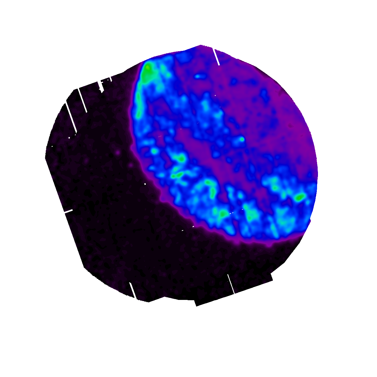
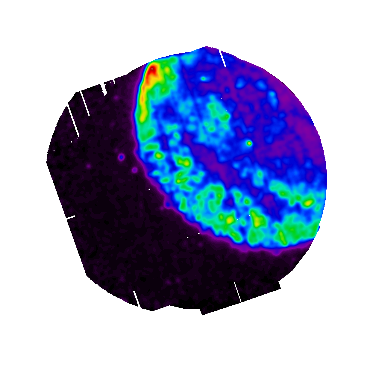
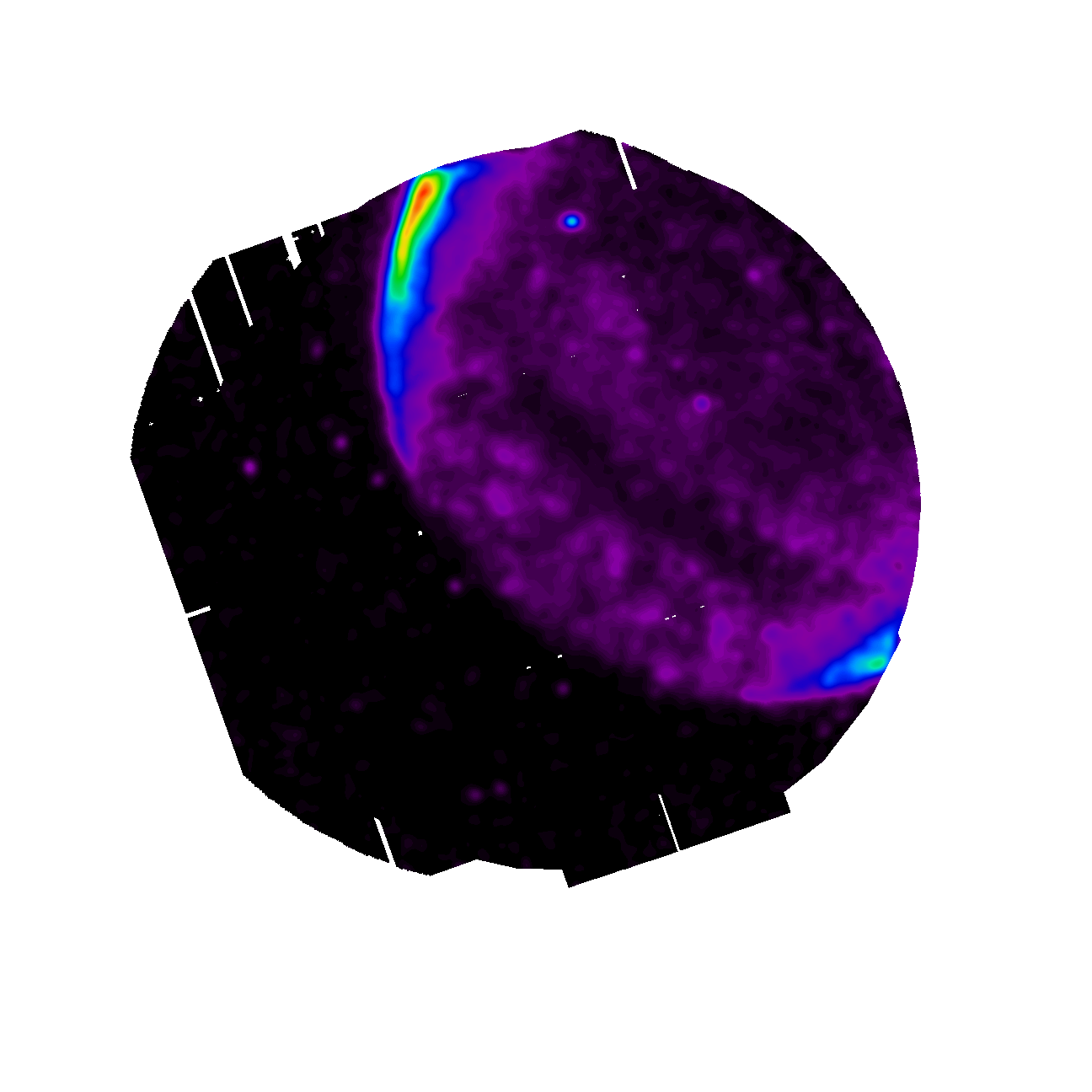
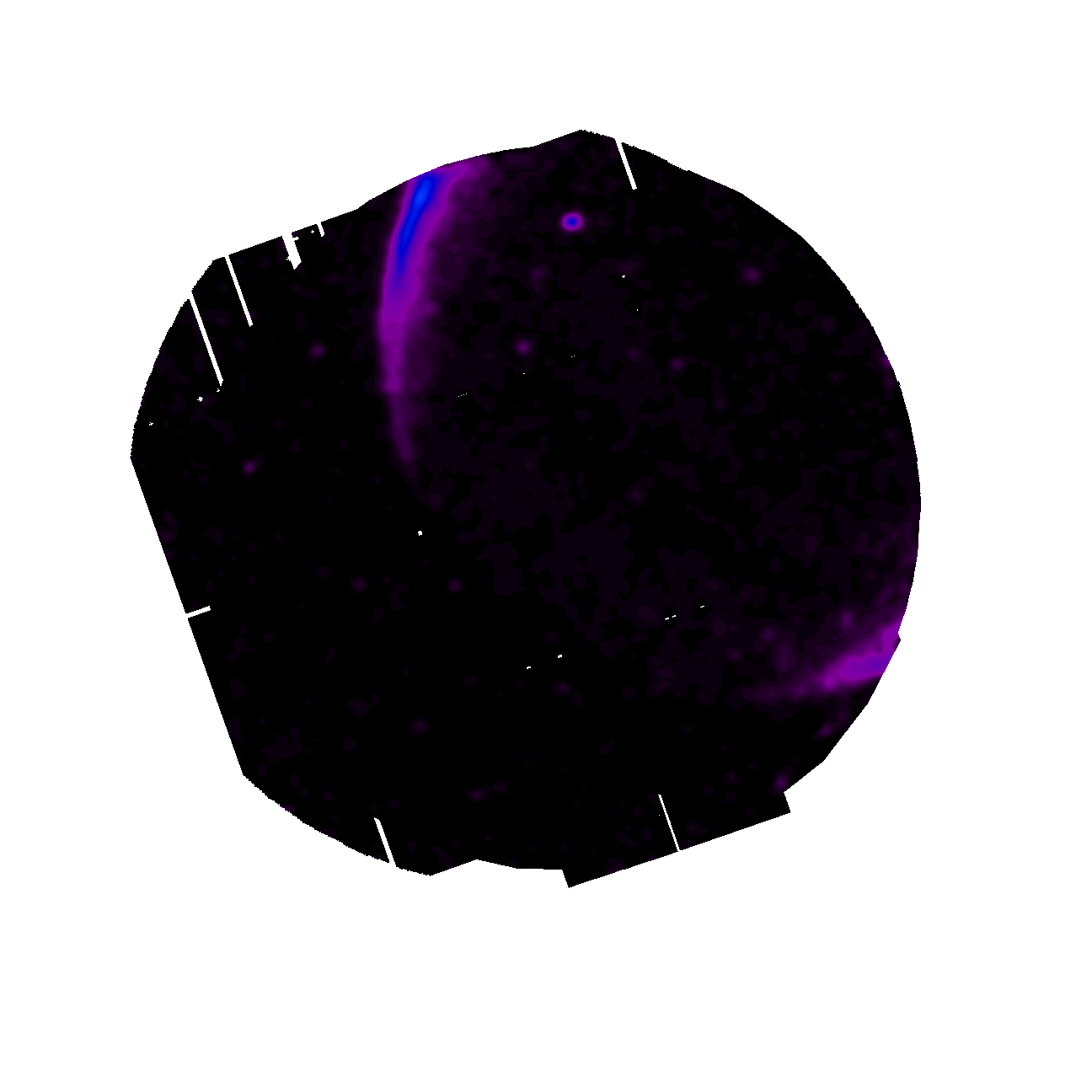
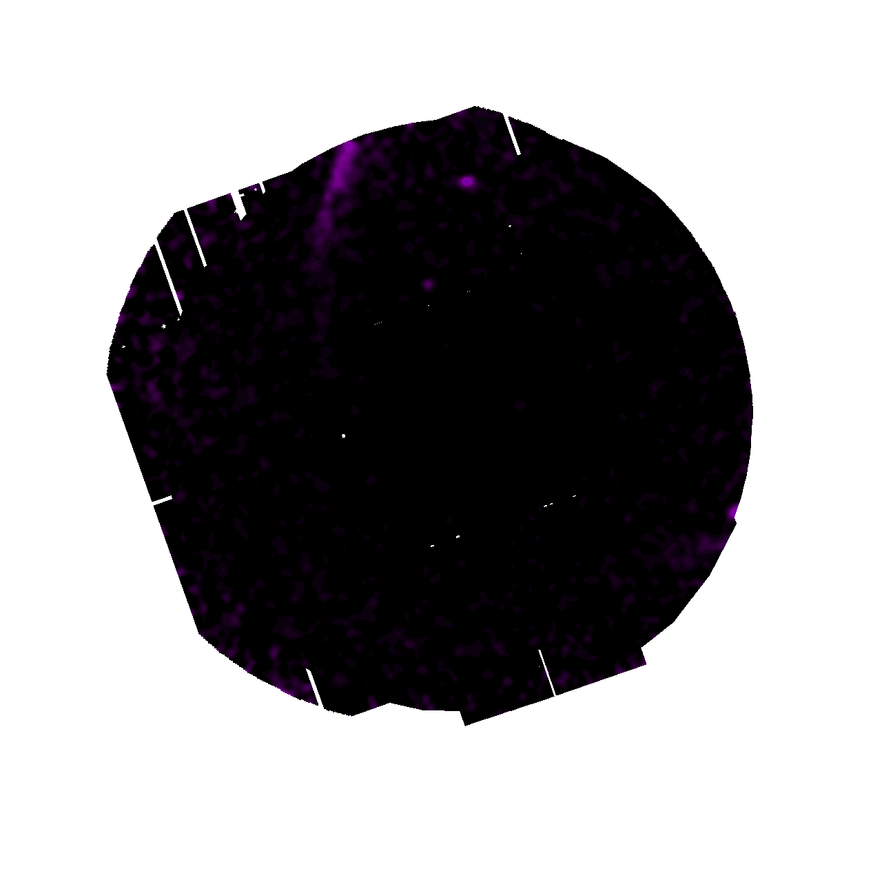
Fig.3: Results of applying eimagecombine to the EPIC science exposure produced by eimageget. The figure shows from top lef to bottom right the final background-subtracted, vignetting-corrected, and smoothed image of the combine EPIC (pn, MOS1 and MOS2) exposures for the five energy ranges considered (0.2-0.5, 0.5-1.0, 1.0-2.0, 2.0-4.5 and 4.5-12.0 keV). The plotting scale of all the images is the same, so images can be visually compared direclty.
|
- Removed a total of (1) style text-align:center;
- Removed a total of (13) style text-align:justify;
- Removed a total of (2) border attribute.
- Converted a total of (5) center to div.