SAS Thread - src find stepbystep - XMM-Newton

EPIC source finding thread: step by step

Procedure
 

This thread illustrates a step-by-step recipe to perform EPIC sources detection. All the individual steps encompassed by the source detection task edetect_chain are commented individually. We stress that a user does not need to run these steps separately, as the input parameters of all the SAS tasks launched by edetect_chain can be set through edetect_chain input parameters. However, some users - in particular SAS novices - may find useful to perform each individual step of the source detection algorithm to achieve a better control and understanding of its outcomes.

In this thread, we will assume that a user intends to detect sources on a single MOS image, extracted in the 0.2-10 keV band.
 

1. Set up your SAS environment (following the SAS start-up thread)
    
2. Create EPIC calibrated event list (see How to reprocess ODFs to generate calibrated and concatenated EPIC event lists). If necessary, create pn and MOS cleaned and filtered for particle background event files for your observation (see  How to filter EPIC event lists for flaring particle background). Let's assume that filtered files have been created, with names: MOS1clean.fits, MOS2clean.fits and PNclean.fits.
    
3. Produce the MOS image in the 0.2-10 keV energy band from the clean calibrated event list (file MOS1clean.evt),
   
      evselect table=MOS1clean.fits:EVENTS imagebinning='binSize' \
        imageset='MOS1_image_full.fits' withimageset=yes xcolumn='X' ycolumn='Y' \
        ximagebinsize=80 yimagebinsize=80 \
        expression='#XMMEA_EM&&(PI in [200:10000])&&(PATTERN in [0:12])'
    
4. Create an exposure map,
   
      eexpmap attitudeset=AttHK.ds eventset=MOS1clean.fits imageset=MOS1_image_full.fits \
        expimageset=MOS1_expmap.ds pimin="200" pimax="10000"
   
   where AttHK.ds is the attitude history file (file *ATT*FIT in the PPS products). An example of exposure map is shown in Fig.1.
    
   
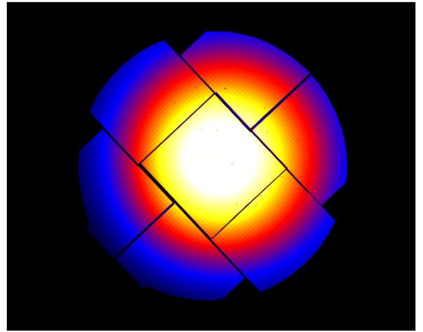
   Fig.1: Example of MOS exposure map
    
5. Create a detection map (masking the areas of the field of view where source detection shall not not be performed),
   
      emask expimageset=MOS1_expmap.ds threshold1=0.25 detmaskset=MOS1_mask.ds
   
   where threshold1 indicates the maximum exposure fraction for a masked pixel (see the emask parameters description). In this specific example all pixels whose exposure time is lower than 0.25 times the maximum exposure are given value "0" in the mask, and excluded from the area where the source detection is performed. Users may relax this choice after a careful look at the exposure map, if they want to seek sources on a larger area.
   
   An example of MOS mask is shown in Fig.2
    
   
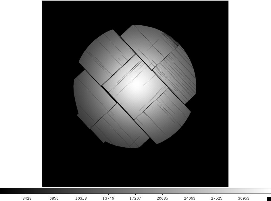
   Fig.2: Example of MOS mask
    
6. Perform a sliding box detection, using locally estimated background,
   
      eboxdetect usemap=no likemin=8 withdetmask=yes detmasksets=MOS1_mask.ds \
        imagesets=MOS1_image_full.fits expimagesets=MOS1_expmap.ds pimin=200 \
        pimax=10000 boxlistset=eboxlist_local.fits
   
   where likemin is the minimum detection likelihood (see the eboxdetect parameters description as well).
    
7. Creating a background map, after masking the sources detected during the previous step,
   
      esplinemap bkgimageset=MOS1_bkg.ds scut=0.005 imageset=MOS1_image_full.fits \
        nsplinenodes=16 withdetmask=yes detmaskset=MOS1_mask.ds withexpimage=yes \
        expimageset=MOS1_expmap.ds boxlistset=eboxlist_local.fits
   
   where nsplinenodes is the number of nodes employed in the background map interpolation and scut the source surface brightness level (in counts per arcseconds squared), above which a source is masked (see the esplinemap parameters description). Particular care needs to be used in the choice of nsplinenodes. A small number of nodes may fail to accurately reproduce the background spatial distribution; an excessive number of nodes may create faked structures. The optimal compromise depends on the spatial pattern of the X-ray emission (background+sources) in a given field of view. Users are encouraged to try different choices for this parameter, and compare the resulting maps with the observed background spatial distribution pattern. The parameter scut mainly drives the amount of source contamination to the interpolated background map, due to the broad wings of the Point Spread Function. The best value of scut is determined by the optimal balance between background integration area and acceptable source contamination level. This is obviously dependent on the amount of background and the on how crowd the field is. Users are encouraged to check the background maps produced by esplinemap for short-scale fluctuations, and tune the scut value accordingly.
   
   An example of MOS background map is shown in Fig.3.
    
   
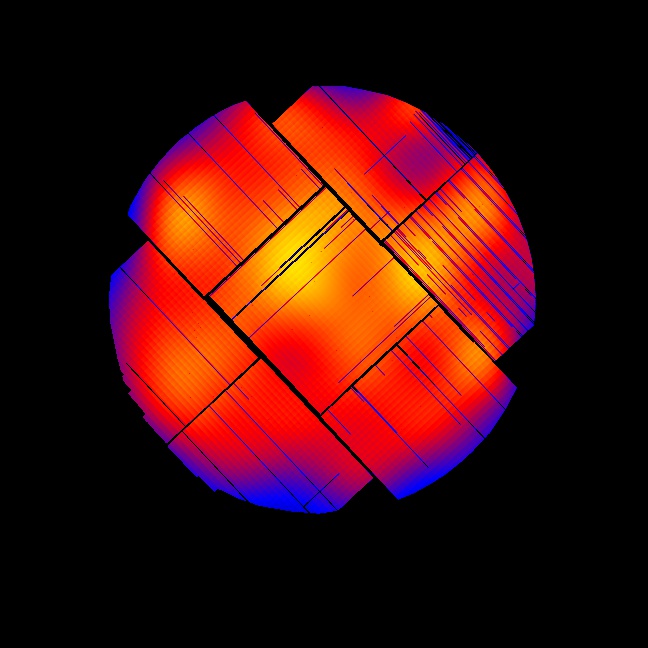
   Fig.3: Example of MOS background map
    
8. Perform a second run of source detection, using the background map calculated during the previous step,
   
      eboxdetect usemap=yes bkgimagesets=MOS1_bkg.ds likemin=8 withdetmask=yes \
        detmasksets=MOS1_mask.ds imagesets=MOS1_image_full.fits \
        expimagesets=MOS1_expmap.ds pimin=200 pimax=10000 boxlistset=eboxlist_map.fits
    
9. Maximum likelihood fitting on the sources detected in the previous step, to,
    
   • optimise source centring (constrained to be the same for all the cameras and/or energy bands, if source detection is performed on multiple images)
   • determine source extend by fitting the local Point Spread Function
   
      emldetect imagesets=MOS1_image_full.fits expimagesets=MOS1_expmap.ds \
        bkgimagesets=MOS1_bkg.ds boxlistset=eboxlist_map.fits ecf=2.0 \
        mllistset=emllist.fits mlmin=10 determineerrors=yes
   
   The ecf is the Energy Conversion Factor to convert count rates (counts/s) to fluxes (10^-11 erg/s/cm²) in a given energy band (a standard definition is reported in Section 6.2.1 of the 3XMM EPIC Source Catalogue User Guide).


10. Create sensitivity maps, i.e. a pixel-by-pixel detection upper limit map,
    
       esensmap expimagesets=MOS1_expmap.ds bkgimagesets=MOS1_bkg.ds \
         detmasksets=MOS1_mask.ds mlmin=10 sensimageset=MOS1_sens_map.fits
    
    An example of MOS sensitivity map is shown in Fig.4.
     
    
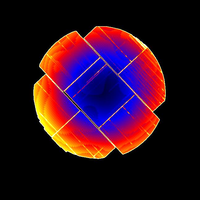
    Fig.4: Example of MOS sensitivity map
     
11. Display the location of the detected sources on the MOS image,
    
       srcdisplay boxlistset=emllist.fits imageset=MOS1_image_full.fits sourceradius=0.01
    
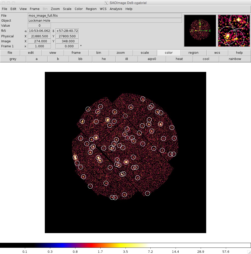      Fig.5: Example of MOS image with detected sources overlaid