
 Sign in
SAS Thread - pn spectrum timing - XMM-Newton
Extraction of pn spectra from point-like sources taken in timing mode
|
Introduction This thread describes how to extract the spectrum of a point-like source observed with the PN camera in timing mode using the command line. Expected Outcome The final outcome of this thread is the standard suite of spectral products required by spectral analysis packages such as XSPEC:
SAS Tasks to be Used Prerequisites
Useful Links
Last Reviewed: 31 January 2025, for SAS v22.0Last Updated: 27 April 2018 |
Procedure
This thread contains a step-by-step recipe to extract PN spectra of a point-like source observed in Timing mode and to create associated response matrices, starting from a calibrated, concatenated event list (produced with epproc / epchain; here it has been assumed that the name of the event file is PN.fits).
All the analysis steps are performed with single SAS tasks started from the command line to explain the general method of generating spectral products and to show explicitly the usage and setting of these task parameters.
- Set up your SAS environment (following the SAS Startup Thread)
- If necessary, create a PN cleaned and filtered for particle background event file for your observation (see the How to filter EPIC event lists for flaring particle background Thread). Let's assume that a filtered file has been created from the file PN.fits, with name: PNclean.fits
- Extract an image in RAW coordinates
evselect table=PNclean.fits imagebinning=binSize imageset=PNimage.fits withimageset=yes \
xcolumn=RAWX ycolumn=RAWY ximagebinsize=1 yimagebinsize=1 - Display the image (Fig.1., left). Note, that in timing mode, the RAWY coordinate is not giving spatial but timing information and hence, the source is visible as a bright strip when plotting RAWX against RAWY.
imgdisplay withimagefile=true imagefile=PNimage.fits
This command is equivalent to the following:
ds9 PNimage.fits
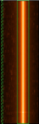
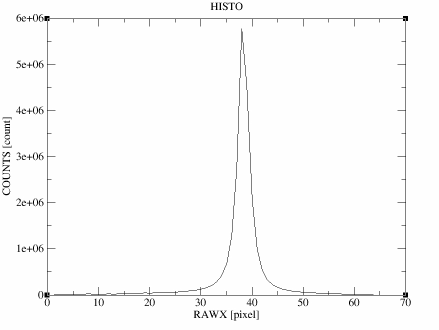
Fig.1: Left, RAWY vs. RAWX image. Rectangular regions have been overlaid to illustrate the source extraction (solid green line) and background extraction (dashed green line) regions. Right, distribution of RAWX (in counts) corresponding to the image on the left. - Select the region, from which the spectrum shall be accumulated. The selection of source and background extraction regions is somewhat arbitrary. In general terms, the source extraction region should be centered in the RAWX column with the highest number of counts. This information can be extracted from the distribution of the RAWX values (Fig.1., right).
Check the Caveats section referring to the treatment of pile-up in timing mode before trying non-standard extraction regions as the ARF generation could not be valid. For example, with the extraction regions illustrated in Fig.1 the use of the xmmselect: Spectral Products generation would be valid.
As for the background region, it should be selected as further away from the source region as possible (see Fig.1., left). For this particular example, the source extraction region is centered in RAWX=38 with a width of 19 pixels. The background region is centered in RAWX=4 with a width of 3 pixels. Have a look at the "EPIC status of calibration and data analysis" document (XMM-SOC-CAL-TN-0018) for latest recommendations on how to select source and background regions.
-
Something that should be kept in mind when defining the source and background extraction regions is that regardeless of the definition given above, the background region can still be contaminated by the source. A good way to see this is by plotting RAWX vs. PI, where PI is the energy of the events in unit of eV (Fig.2.). Notice that the effect is energy dependant (refer to XMM-SOC-CAL-TN-0083 for more information).
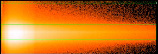
Fig.2: RAWX vs. PI image. PI has been limited between 0.2-10. keV to produce this image. The scale in the z-axis has been set to logarithmic to enhance the effect. The solid and dashed green boxes overlaid on the image correspond to the same source and background extraction regions used in Fig.1. Other useful information on the selection of source and background extraction regions can be found in the Caveats section and in the SAS User Guide (EPIC chapter, section titled Generating spectra).
- Extract a source spectrum, using the region highlighted in Fig.1, left, and restricting the patterns to single and double events. It is important to check withspecranges and use the following spectral bin range, specchannelmin=0 and specchannelmax=20479, to accumulate the spectrum (see Caveats).
evselect table=PNclean.fits withspectrumset=yes spectrumset=PNsource_spectrum.fits \
energycolumn=PI spectralbinsize=5 withspecranges=yes specchannelmin=0 specchannelmax=20479 \
expression='(FLAG==0) && (PATTERN<=4) && (RAWX>=29) && (RAWX<=47)' - Extract a background spectrum, using the region highlighted in Fig.1., left. In the following, we assume that the background is extracted from a source-free region.
evselect table=PNclean.fits withspectrumset=yes spectrumset=PNbackground_spectrum.fits \
energycolumn=PI spectralbinsize=5 withspecranges=yes specchannelmin=0 specchannelmax=20479 \
expression='(FLAG==0) && (PATTERN<=4) && (RAWX>=3) && (RAWX<=5)' - Calculate the area of source and background region used to make the spectral files. The area is written into the header of the spectrum table of the file as keyword BACKSCAL (if the spectrum is created via xmmselect, backscale will run automatically) (see Caveats).
backscale spectrumset=PNsource_spectrum.fits badpixlocation=PNclean.fits
backscale spectrumset=PNbackground_spectrum.fits badpixlocation=PNclean.fits - Generate a redistribution matrix
Currently there are two possible approaches:
a) use the SAS task rmfgen to create a redistribution matrix for your previously extracted spectrum:
rmfgen spectrumset=PNsource_spectrum.fits rmfset=PN.rmfb) use the ready-made (canned) response matrix.
- Generate an ancillary file
arfgen spectrumset=PNsource_spectrum.fits arfset=PN.arf withrmfset=yes rmfset=PN.rmf \
badpixlocation=PNclean.fits detmaptype=psf
- Rebin the spectrum and populate the header keywords with the names of the required response and background files. In the following example the spectrum is rebinned in order to have at least 25 counts for each background-subtracted spectral channel and not to oversample the intrinsic energy resolution by a factor larger than 3.
specgroup spectrumset=PNsource_spectrum.fits mincounts=25 oversample=3 rmfset=PN.rmf \
arfset=PN.arf backgndset=PNbackground_spectrum.fits groupedset=PN_spectrum_grp.fits
The rebinning options shown in the example above, are by no means the only possible binning available, or the recommended one; more binning options are available in the description of the task specgroup.
- Fit the grouped spectrum: PN_spectrum_grp.fits
|
To extract a spectrum, withspecranges must be checked (set to yes), with specchannelmin set to 0, and specchannelmax set to 20479 for the PN. It is important to use this PI range. Selecting a spectrum with a non-standard PI range results in wrong response matrices with an impact on any spectral results derived when using them. If a spectrum needs to be generated within a given energy range, this must be done through the selection expression and not by changing the PI range through specchannelmin and specchannelmax. As of SAS v13.5, users should no longer run the epfast task for Timing mode data processing. As of SAS v16.1, an issue has been identified with running the backscale task for PN Timing Mode spectral analysis. Please refer to the corresponding watchout item for a detail desciption on the issue. This problem has been fixed in arfgen v1.96 and backscale v1.6 (SAS v18) by implementing the parameter badpixelresolution. If your observation is affected by pile-up, check the corresponding section of the SAS User Guide (EPIC chapter, section How to analyse a piled-up Timing mode observation) for information on the analysis of piled-up Timing mode observations. Of especial relevance is the recipe on how to deal with the generation of an ARF file using the SAS task arfgen. See also the thread on How to evaluate the pile-up fraction in an EPIC source. Notice that in the case of PN Timing mode observations (where the rate of single to double events depends on the source position) one should always create and fit a spectrum of the combined single and double events. For more details on the spectral analysis of data obtained in Timing and Burst mode, see XMM-SOC-CAL-TN-0018. Timing mode is typically used to observe bright sources. This means that the counts from the whole CCD area are dominated by the source, leaving often no source free-region areas from which the background can be reliably obtained. In such a case, it might be better not to perform any background subtraction. Users are referred to the discussion in XMM-SOC-CAL-TN-0083. For observations taken in pn burst mode, users are referred to the document XMM-SOC-CAL-TN-0069, where the special techniques of data reduction needed for this mode are described. |
- Removed a total of (1) style text-align:center;
- Removed a total of (15) style text-align:justify;
- Removed a total of (9) align=center.
- Removed a total of (4) border attribute.
- Converted a total of (4) center to div.