SAS Thread - xspec - XMM-Newton

XSPEC Session Thread

Procedure
 

This thread contains a (very!) simple standard XSPEC session for fitting data from the XMM-Newton X-ray and optical cameras.

EPIC
 

The EPIC case will be illustrated with an EPIC-pn spectrum (a fully analogous procedure applies to EPIC-MOS spectra as well). We assume in the following that the products have been created and are available in the working directory: a source+background spectrum (PNspectrum.pi), a background only spectrum (PNspectrum_background.pi), a redistribution matrix (PN.rmf), and an ancillary file (PN.arf), both of the later appropriate for the source+background spectrum in use (see Prerequisites for this thread at the top of the page on how to create the spectra and associated files for point-like sources with EPIC-pn or EPIC-MOS). We also assume that the spectrum keywords are not already populated with the response and background files using tasks such as specgroup.

1. Start XSPEC
   
    xspec
    
2. Load spectrum data
   
    data 1 PNspectrum.pi
    
3. Load the background spectrum
   
    backgrnd 1 PNspectrum_background.pi
    
4. Load the redistribution matrix
   
    response 1 PN.rmf
    
5. Load the ancillary file
   
    arf 1 PN.arf
    
6. Create the output graphic plotting window
   
    cpd /xs
    
7. Define how data has to be plotted, e.g. in energy bins (wavelength would be a valid alternative)
   
    setplot energy
    
8. Ignore bad channels in data
   
    ignore bad
    
9. Ignore energy intervals where the pn matrices are currently not calibrated (e.g. beyond the energy band 0.2-15.0 keV)
   
    ignore **-0.2 15.-**
   
   (check the EPIC Calibration Status Document for recommended energy ranges to be used for the different modes and EPIC instruments)
    
10. Relax getting a look into your data
    
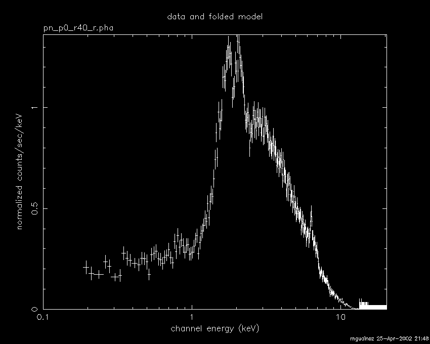
     plot data
     
    
    Fig.1: XSPEC data plot
     
11. Load a model to be fitted (in this case a simple power law model with photoelectric absorption)
    
     model wabs*powerlaw
    
    (you will have to hit return several times for every parameter of the model). The following screen will appear:
     

     mo = wa((po)).
      Model:  wabs[1]( powerlaw[2] )
    Input parameter value, delta, min, bot, top, and max values for ...
    Current:           1     0.001         0         0     1E+05     1E+06
    wabs:nH>
    Current:           1      0.01        -3        -2         9        10
    powerlaw:PhoIndex>
    Current:           1      0.01         0         0     1E+24     1E+24
    powerlaw:norm>
      ---------------------------------------------------------------------------
      ---------------------------------------------------------------------------
      Model:  wabs[1]( powerlaw[2] )
      Model Fit Model Component  Parameter  Unit     Value
      par   par comp
        1    1    1   wabs       nH       10^22      1.000     +/-      0.
        2    2    2   powerlaw   PhoIndex            1.000     +/-      0.
        3    3    2   powerlaw   norm                1.000     +/-      0.
      ---------------------------------------------------------------------------
      ---------------------------------------------------------------------------
     Chi-Squared =     2.7158111E+09 using  1675 PHA bins.
     Reduced chi-squared =      1624289.     for   1672 degrees of freedom
     Null hypothesis probability =    0.
    

12. Fit the parameters
    
     fit 100 1e-1
    
    The former number indicates the maximum number of iterations before the minimization routine stops. The latter number indicates the difference in fit statistic between iterations below which the fit is deemed to have converged.


13. Set the rebinning of your choice (for plotting purposes only!)
    
     setplot rebin 3 4096
    
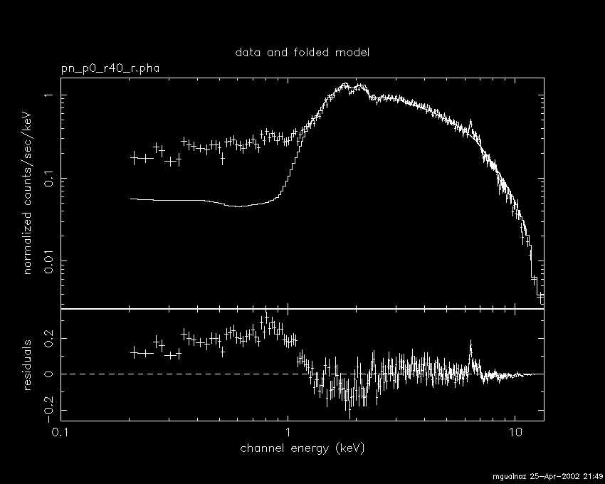
    The former number indicates the maximum number of sigma to be accumulated in a rebinned channel; the latter, the maximum number of channels to be summed.


14. Plot the data with the model adjustment and e.g. the residuals (alternatives, ratio data/model, absolute chi-squared, etc)
    
     plot data residuals
     
    
    Fig.2: XSPEC data, model and residual plot
     
15. Determine one-side errors on the best-fit parameters 1, 2 and 3
    
     error 2.706 1 2 3
    
    The first number indicates the delta chi-squared value.
     

RGS
 

We will assume in the following that products are available in the work directory as produced by SAS rgsproc, the RGS SAS metatask for whole data reduction (see Prerequisites for this thread at the top of the page on how to extract RGS spectra of a point-like source and associated matrices):

1. Start XSPEC
   
    xspec
    
2. Load the spectrum data (in this case the RGS1 first order spectrum) into the first internal dataset
   
    data 1:1 /xvsas05/sasval/data/procred/Mkn421/P0099280201R1S001SRSPEC1001.FIT
    
3. Load the corresponding background file:
   
    backgrnd 1 /xvsas05/sasval/data/procred/Mkn421/P0099280201R1S001BGSPEC1001.FIT
    
4. Load the response matrix into the first internal response set. The SAS task rgsrmfgen puts both response and ancillary data into the response matrix file
   
    resp 1 /xvsas05/sasval/data/procred/Mkn421/P0099280201R1S001RSPMAT1001.FIT
    
5. Loading a second dataset into second internal data position (in this case data corresponding to RGS2)
   
    data 2:2 /xvsas05/sasval/data/procred/Mkn421/P0099280201R2S002SRSPEC1001.FIT
    
6. Load the corresponding background file:
   
    backgrnd 2 /xvsas05/sasval/data/procred/Mkn421/P0099280201R2S002BGSPEC1001.FIT
    
7. Load the corresponding response matrix
   
    resp 2 /xvsas05/sasval/data/procred/Mkn421/P0099280201R2S002RSPMAT1001.FIT
   
   A few differences need to be noticed at the data loading level:
    
   • rgsrmfgen (the SAS tasks to generate RGS response matrices, which is run by default in the last stage of rgsproc) creates a response matrix which includes both the redistribution matrix and the effective area vector (ancillary file). There is therefore no need to load any *.arf files in XSPEC when analyzing RGS spectra
      
   • The syntax data n:n allows to keep the fit parameter (fully or partly) independent between the two datasets during the fitting procedure. The alternative syntax data n forces the same model parameters to be fitted to all datasets
      
8. Create the output graphic plotting window
   
    cpd /xs
    
9. Define how the data has to be plotted, e.g. in energy bins (wavelength would be a valid alternative)
   
    setplot energy
    
10. Relax getting a look into your data
    
     plot data
     
11. Ignore bad channels in data
    
     ignore bad
     
12. Ignore energy intervals where the RGS matrices are currently not calibrated (e.g.: beyond 1.9 keV)
    
     ignore 1.9-**
     
13. Load a model to be fitted (in this case a simple power law model)
    
     model powerlaw
    
    (you will have to hit return several times for every parameter of the model)
     
14. Fit the parameters
    
     fit 100 1e-1
    
    The former number indicates the maximum number of iterations before the minimization routine stops. The latter number indicates the difference in fit statistic between iterations below which the fit is deemed to have converged. 
     
15. Set the rebinning of your choice (for plotting purposes only!)
    
     setplot rebin 3 4096
    
    The former number indicates the maximum number of sigma to be accumulated in a rebinned channel. The latter, the maximum number of channels to be summed.
     
16. Plot the data with the model adjustment and e.g the residuals  (alternatives, ratio data/model, absolute chi-squared, etc)
    
     plot data residuals
     

Notice that the help system in XSPEC is started with help.

OM
 

In order to analyse an OM spectrum with XSPEC, we need: (1) the output spectrum of the task om2pha (see Converting OM data to OGIP II format); (2) the canned response files, one for each filter, that can be downloaded from the XMM-Newton OM response files page. The task om2pha already populated the header keywords of the OM spectrum with the response files names, so there is no need to explicitely insert them in XSPEC. However, in order for the keywords to be read properly by XSPEC, the name of the corresponding canned response files do not have to be changed. Moreover, the files need to be located in the same directory as the OM spectrum. In the following example, we will load simulatenously PN and OM spectra.

1. Start XSPEC
   
    xspec
    
2. Load the EPIC-pn spectrum data
   
    data 1:1 PNspectrum.pi
    
3. Load the EPIC-pn background spectrum data
   
    background 1 PNspectrum_background.pi
    
4. Load the EPIC-pn redistribution matrix
   
    response 1 PN.rmf
    
5. Load the EPIC-pn ancillary file
   
    arf 1 PN.arf
    
6. Load the OM spectrum data (that in this case has six filters)
   
    data 1:2 OMspectrum.pi{1-6}
    
7. Ignore bad channels in data
   
    ignore bad
    
8. Ignore energy intervals where the EPIC-pn matrices are currently not calibrated (e.g. beyond the energy band 0.2-15.0 keV)
   
    ignore 1 **-0.2 15.-**
    
9. Create the output graphic plotting window
   
    cpd /xs
    
10. Define how the data has to be plotted, e.g. in energy bins (wavelength would be a valid alternative)
    
     setplot energy
     
11. Plot the data, e.g. in logarithmic scale
    
     plot ldata
     
    
    Fig.3: XSPEC logarithmic data of EPIC-pn and OM spectra
     
12. Proceed loading the model and fitting as described above for EPIC and RGS.