SAS Thread - evenergyshift - XMM-Newton

CORRECT FOR RATE-DEPENDENT ENERGY SCALE EFFECTS IN pn BURST AND TIMING MODE

Procedure

This thread contains a step-by-step procedure to analyse the spectrum of an EPIC-pn observation in Timing or Burst mode, estimate the energy shift necessary to eliminate or reduce possible spectral residuals around instrumental edges, and create a modified event file with the observation-specific energy scale correction applied.

The steps to follow in general terms are:

• Reduce the data with the default processing (which includes the RDPHA correction), and extract the spectrum (if the observation is affected by pile-up, see the Caveats section below);

• With XSPEC, check the residuals in the energy spectrum around the instrumental edges at 1.8 keV, 2.2 keV and 11.9 keV;

• If there are significant residuals around one or more edges, isolate each of those instrumental edges and use the XSPEC command gain fit to find the energy shift necessary to reduce the residuals resulting from the default calibration;

• Apply the resulting energy shift associated with each edge to the event file with the SAS task evenergyshift to create a corrected event file;

• From the newly created, corrected event file, re-extract the energy spectrum and proceed with the spectral analysis.

We will detail here the case for an EPIC-pn observation made in Timing mode. For Burst mode observations the user can follow the same steps.

It is assumed that an event file called pn-events.fits already exists, from which an energy spectrum pn-spectrum.pi, a background spectrum pn-bkd-spectrum.pi and ancillary and response files pn.arf and pn.rmf, have been extracted.

With those four files, we can enter XSPEC to explore the spectrum and apply the corrections if necessary. Follow the steps below.
 

1. Start XSPEC
   
    xspec
    
2. Load the source spectrum
   
    data 1 data pn-spectrum.pi
    
3. Load the background spectrum
   
    backgrnd 1 background pn-bkd-spectrum.pi
    
4. Load the redistribution matrix
   
    response 1 response pn.rmf
    
5. Load the ancillary file
   
    arf 1 arf pn.arf
    
6. Create the output graphic plotting window
   
    cpd /xs
    
7. Define how data has to be plotted (in this case energy scale)
   
    setplot energy
    
8. Ignore bad channels in data
   
    ignore bad
    
9. Ignore energy intervals where the pn matrices are currently not calibrated (e.g. beyond the energy band 0.2-15.0 keV)
   
    ignore **-0.2 15.-**
   
   (check the EPIC Calibration Status Document for recommended energy ranges to be used for the different modes and EPIC instruments)
    
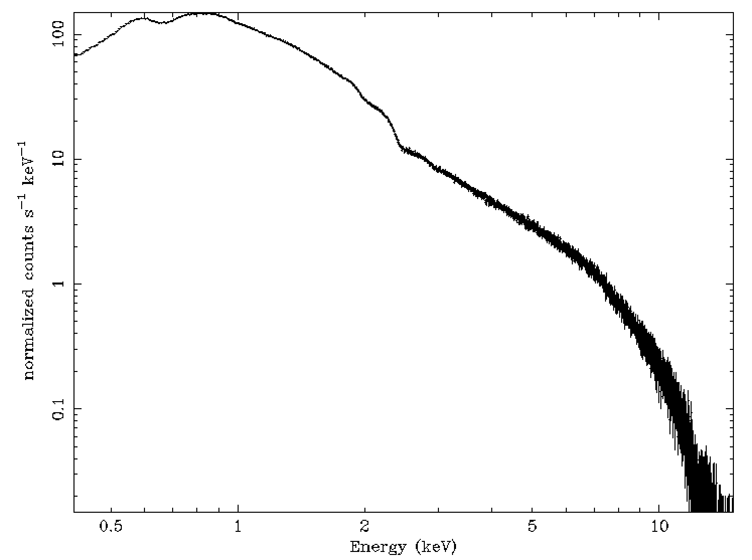
10. Plot and inspect the data
    
     plot ldata
     

    

11. Load the model to be fitted (in this case a simple power law model with photoelectric absorption)
    
     model tbabs*po
     
12. Fit the parameters
    
     fit 100 1e-1
     

    The former number indicates the maximum number of iterations before the minimization routine stops. The latter number indicates the difference in fit statistic between iterations below which the fit is deemed to have converged.

13. Now examine the residuals at the instrumental edges, in this example the Au M-edge at 2.2 keV. For that, ignore the following energy intervals
    
     ig **-1.8
     ig 2.8-**
     
14. Plot the narrowed energy range (it can be useful to plot in channel space, as is done here) with the current model and residuals
    
     setplot ch
     plot ldata de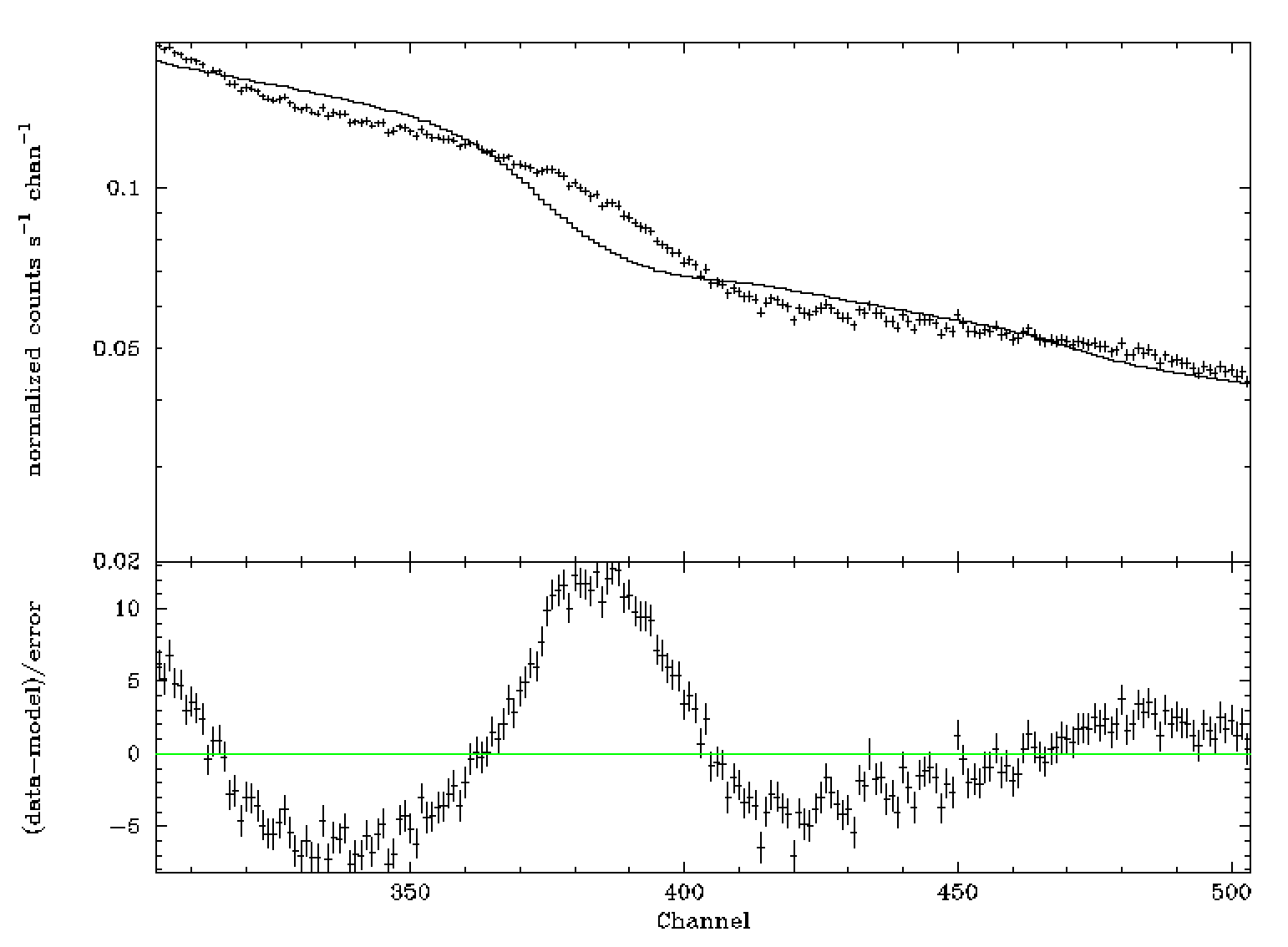

    

    If there are significant residuals (as in this example above), this could be an indication of a not fully correted energy scale in the default processing.

15. Quantify the shift in energy scale required to minimise these residuals, using the XSPEC command gain fit
    
     gain fit
     
16. You will be prompted for the initial values of the slope and the offset of the gain correction - the slope should be fixed to 1, the offset should be a free parameter
     
    • Enter 1,-1 for the slope, thus making it a fixed parameter.
    • Hit return for the offset, making it a free parameter.
       
17. Refit the data and derive the model parameters along with the best-fitting offset, which will be listed as the last parameter
    
     fit 100 1e-1
     plot ldata de
    
     

    

    

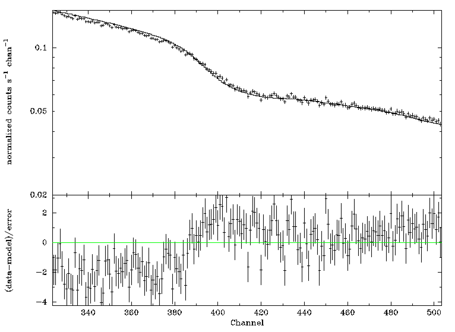
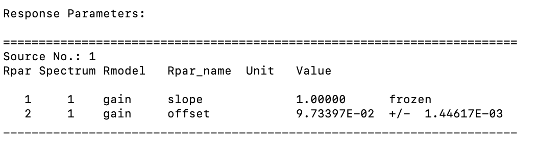
    Note the gain offset value representing the energy shift corresponding to this instrumental edge. Repeat the same procedure for the edges at 1.8 keV and 11.9 keV (if meaningful).

18. Now one may quit XSPEC
    
     exit

Once we finished with XSPEC, the SAS task evenergyshift can be used to create an events file with the energy shifts derived above applied. Regarding the values passed, please note:

• the gain offset and corresponding edge energies should be expressed as integer eV, and
• the gain offset value should change sign (due to the different interpretation of the offset in XSPEC and evenergyshift)

In this example, the task would be called as follows:

  evenergyshift table=pn-events.fit \
   outset=pn-events-modified.fits pi1=2200 offset1=-97

this will apply an energy shift of -97 eV to all event energies.

If energy shifts are required at other instrumental edges, the call would be, e.g.:

  evenergyshift table=pn-events.fits \
   outset=pn-events-modified.fits pi1=1800 offset1=-50 pi2=2200 offset2=-97

In such cases, i.e. where different energy offset values (offset1, offset2, ...) are passed at multiple energies (pi1, pi2, ...), the default behaviour of evenergyshift is to apply energy shifts by linearly interpolating offset values between successive pi values, and extrapolating the trend beyond the highest pi value.

As mentioned, the default behaviour is to extrapolate the trend beyond the highest pi value, however, the extrapolation can be swiched off by passing the option extrapolate=no. In this case beyond the highest pi value a constant is assumed.

The resulting modified events file, pn-events-modified.fits, can now be used to re-extract the energy spectrum.