SAS Thread - timing gui - XMM-Newton

Extraction and correction of an X-ray light curve for a point-like source (GUI version)

Procedure

EPIC
 

The content of this thread is the same as Extraction and correction of an X-ray light curve for a point-like source (command-line version). Here, however, the extraction of scientific products is being done using the SAS task xmmselect. This is a user-friendly, graphical interface to the SAS extractor (evselect), which allows you to create a wide range of scientific products (images and pseudo-images, time series, spectra, histograms), and screen the data prior to any product accumulations. xmmselect takes advantage of the full integration between SAS and tools such as grace and ds9, to define data selection regions on a 1-D (light curve) or 2-D (image) plane.

As an example case, we will consider the extraction of a light curve from a pn event list (PN_evt.fits). The same recipe applies for MOS.

1. Set up your SAS environment (see Prerequisites for this thread at the top of the page).
    
2. If necessary, create a PN cleaned and filtered for particle background event file for your observation (see the How to filter EPIC event lists for flaring particle background Thread). Let's assume that a filtered file has been created, with name: PNclean.fits
    
3. Be aware: if you are interested in very short time periods, such as they appear in pulsars or cataclysmic variables, you have to perform a barycentric correction. This means that the arrival time of a photon is shifted as is it would have been detected at the barycentre of the solar system (the centre of mass) instead at the position of the satellite. In this way, the data are comparable. The SAS task barycen performs this correction. As barycen overwrites the TIME column entries, it is advisable first to copy the original event list and keep it as a backup.
   
   cp PNclean.fits PNclean_nobarycen_cor.fits
   barycen table=PNclean.fits:EVENTS
    
4. Start xmmselect
   
   xmmselect table=PNclean.fits &
   
   First a window pops-up, asking if you wish to visualize the "[...] selection expression [...]" corresponding to "[...] data subspace information [...]". In practice, xmmselect is asking you if you wish to see the data screening expression, which was employed to generate the event list. The answer to this question does not affect the following steps.
   
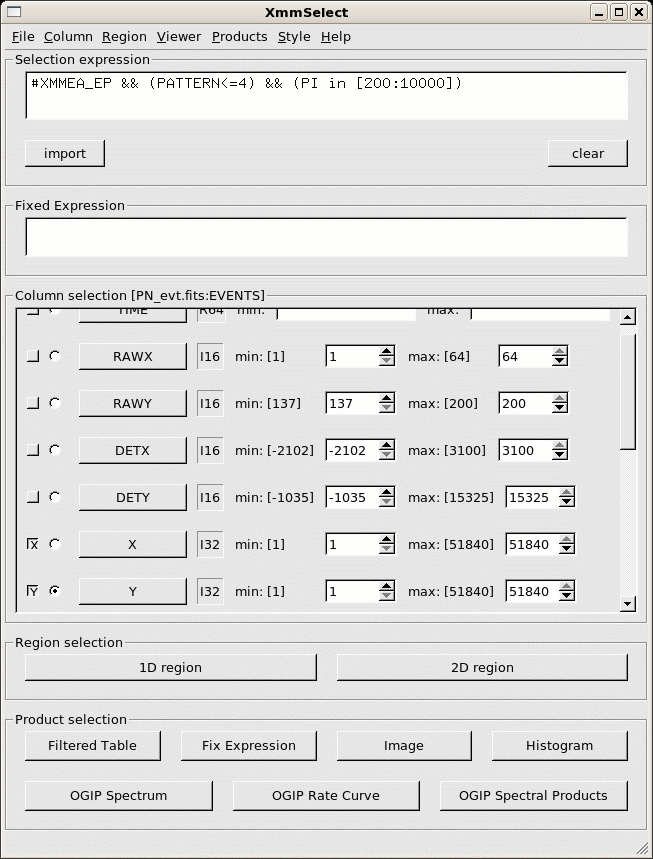
   The xmmselect call pops-up a window as shown in Fig.1.
    
   
   Fig.1: The main xmmselect window.
   
   In this window, we identify:
    
   • a data screening widget (top)
   • a data column panel (middle)
   • the buttons 1D region and 2D region, which allow to translate selection expressions defined in a grace or ds9 window, respectively, into proper selectlib expressions
   • "action" buttons (bottom)
   
   As customary for SAS tasks, each widget, button or menu in the evselect window corresponds to a task parameter. The whole list of available evselect parameters, with their description, is available at the evselect task description.
    
5. Filter the events with a quality selection appropriate for a later light curve extraction as one shown for PN in the xmmselect window of Fig.1: #XMMEA_EP && (PATTERN<=4) && (PI in [200:10000]), taking good events, singles and doubles with an energy range between 200 and 10000 eV (corresponding MOS selection would be #XMMEA_EM && (PATTERN<=12) && (PI in [200:10000])). Extract an image (sky coordinates in this example; extraction in detector - DET[XY] - coordinates is possible as well). This is accomplished by:
    
   • clicking the square check boxes beside X and Y in the data column xmmselect panel
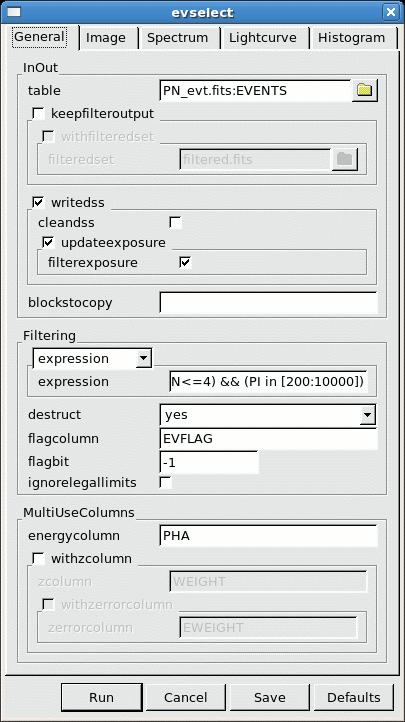
   • click on Image. This will pop-up another window: the evselect parameter user interface (see Fig.2)
     
      
     
     Fig.2: The main evselect window
      
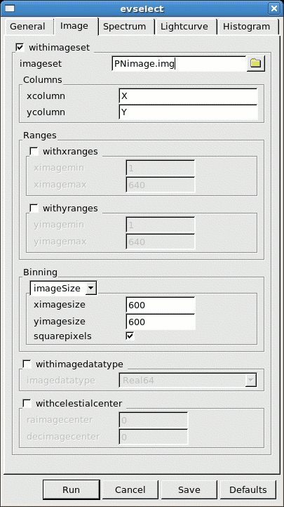
   • go to the Image panel in the evselect window (see Fig.3)
     
      
     
     Fig.3: The Image panel in the evselect window
      
   • change at least the file name in the imageset window (e.g. to PNimage.img)
   • click Run
   
   xmmselect will automatically launch a ds9 window on the created image (Fig.4)
    
6. Select the region, from which the source light curve shall be accumulated, using the Regions/Shape/Circle in ds9 (see Fig.4). Have a look at the "EPIC status of calibration and data analysis" document (XMM-SOC-CAL-TN-0018) for latest recommendations on how to select source and background regions.
    
   
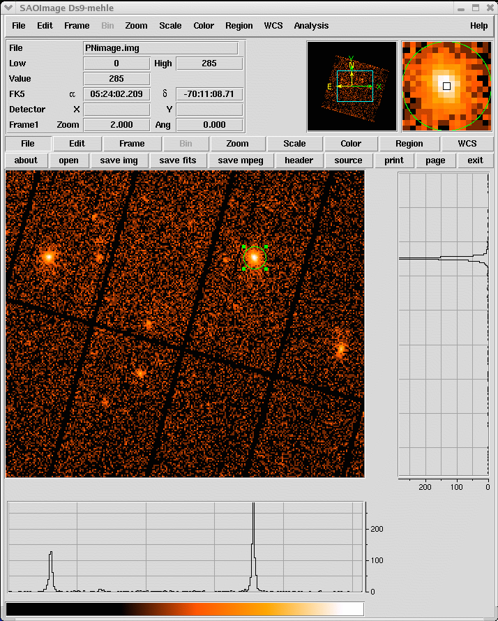
   Fig.4: ds9 main window. A circular region (green circle) has been defined using the highlighted menu.
    
7. Propagate the selected region into the xmmselect data screening panel, by clicking the 2D region button.
    
8. Extract a light curve in the spatial region defined by the previous 2 steps, restricting the accumulation to single and double events, and the energy range between 200 and 10000 eV.
    
   • click the circular check box close to TIME in the data column xmmselect panel
   • click OGIP Rate Curve
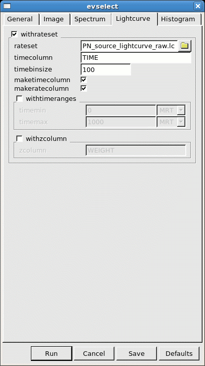
   • go the the Lightcurve panel in the evselect window (see Fig.5)
      
     
     Fig.5: The Lightcurve panel in the evselect window
      
   • define the parameters:
      
     • withrateset active
     • rateset=PN_source_lightcurve_raw.lc
     • timecolumn=TIME
     • timebinsize=100
     • maketimecolumn active
     • makeratecolumn active
     
     The last two parameters tell evselect to generate a light curve in count rates, and a column TIME in the output file.
      
   • click Run
      
   xmmselect launches automatically a grace window, displaying the output light curve (as shown for background light curve in Fig.6)
    
   
   Fig.6: the grace panel displaying the light curve
    
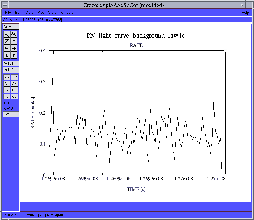
9. Extract a background light curve (PN_light_curve_background_raw.lc) from a region of the PN field-of-view free from contaminating sources, using the same steps 4. to 6. above. Have a look at the "EPIC status of calibration and data analysis" document (XMM-SOC-CAL-TN-0018) for the latest recommendations on how to select source and background regions. At minimum, the background should be extracted from a source-free region at the same distance to the readout node (RAWY position) as the source region. If this is not possible, in order to ensure a similar low-energy noise contribution, you should aim to select the background from the same CCD or same quadrant of the source region.
    
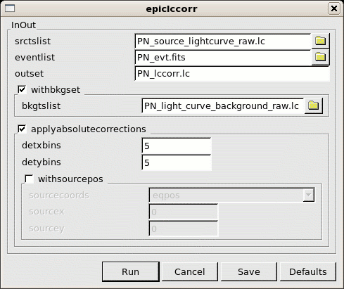
10. However, light curves obtained in such a way should be corrected for diverse effects affecting the detection efficiency, such as vignetting, bad pixels, PSF variation and quantum efficiency, as well as for variations affecting the stability of the detection within the exposure, like dead time and GTIs. Since all these effects can affect in a different manner source and background light curves, the background subtraction has to be done accordingly. A SAS task, epiclccorr, performs all of these corrections at once. It requires as input both light curves (which are used to establish the binning of the final corrected background subtracted light curve) and the event file, therefore subtract the background from the source lightcurve with epiclccorr
     
    • launch epiclccorr -d
    • defining the proper parameters (Fig.7):
       
      
      Fig.7: The epiclccorr window
       
      • srctslist to the file name of the source light curve (PN_source_lightcurve_raw.lc)
      • eventset to the file name of the event list (PN_evt.fits)
      • outset to the name of the output file (PN_lccorr.lc)
      • withbkgset active
      • bkgtslist to the file name of the background light curve (PN_light_curve_background_raw.lc)
      • applyabsolutecorrections yes
         
    • click Run
       
11. Plot the resulting light curves, e.g.
    
    dsplot table=PN_lccorr.lc withx=yes x=TIME withy=yes y=RATE
    
    This command will launch the following xmgrace window.
     
    
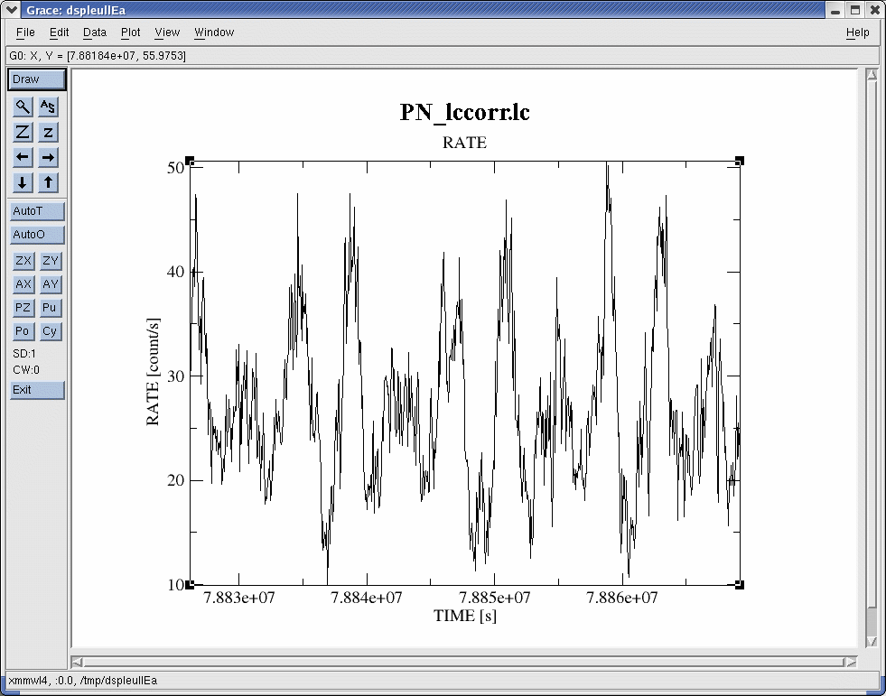
    Fig.8: xmgrace window, containing the background-subtracted exposure-corrected light curve.
    
    The file PN_lccorr.lc contains the background-subtracted exposure corrected light curve. This file is compliant with the OGIP standards, and therefore can be processed by, e.g., the XRONOS package (refer to the Timing Analysis Thread if you want to continue this way).

RGS
 

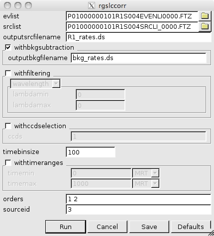
We will assume in what follows that RGS products are available in the working directory: a) RGS event list; b) RGS source list (following the How to reduce RGS data and extract spectra of point-like sources thread). A call to the task rgslccorr will perform light curve extraction, correction and background subtraction using events from the same selection regions used for extraction of spectra for both source and background.
 

1. Create, for example, a combined RGS1 and RGS2, 1st and 2nd order, 100-second binned exposure-corrected and background-subtracted light curve, for the 3rd source in the source list
   
   rgslccorr -d
    
   
   Fig.9: the rgslccorr GUI window.


2. After rgsclccorr has ran, plot the resulting light curves, for example,
   
   dsplot table=R1_rates.ds withx=yes x=TIME withy=yes y=RATE
   
   This command will launch the following xmgrace window with the combined RGS light curve.
    
   
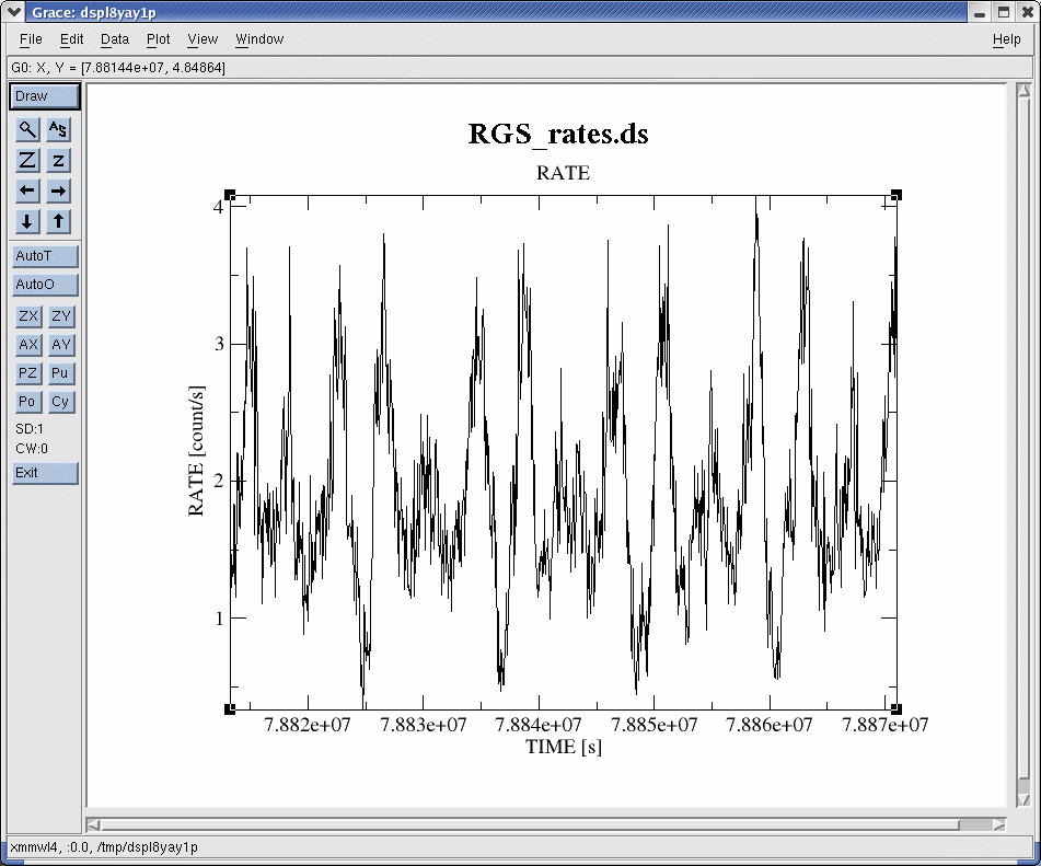
   Fig.3: xmgrace window showing the background-subtracted exposure-corrected RGS light curve.