SAS Thread - background - XMM-Newton

How to use EPIC instrumental background files

Procedure
 

1. Set up your SAS environment (see Prerequisites for this thread at the top of the page).
    
2. Create EPIC event files for your science observation (see Prerequisites for this thread at the top of the page). The name of the event files that will be used in this thread for obsid 0555630101 are:
   
      1594_0555630101_EPN_S003_ImagingEvts.ds
      1594_0555630101_EMOS1_S001_ImagingEvts.ds
      1594_0555630101_EMOS2_S002_ImagingEvts.ds
   
   with Livetimes, 3.44e+04 sec, 4.49e+04 sec and 4.49e+04 sec respectively.
    
3. Run the SAS task evqpb over each one of these event files.
   
      evqpb table=1594_0555630101_EPN_S003_ImagingEvts.ds exposurefactor=2.0 \
          attfile=1594_0555630101_AttHk.ds outset=evqpb_pn.fits
   
      evqpb table=1594_0555630101_EMOS1_S001_ImagingEvts.ds exposurefactor=2.0 \
           attfile=1594_0555630101_AttHk.ds outset=evqpb_m1.fits
   
      evqpb table=1594_0555630101_EMOS2_S002_ImagingEvts.ds exposurefactor=2.0 \
           attfile=1594_0555630101_AttHk.ds outset=evqpb_m2.fits
    

   To generate the output FWC event file, events from the repository are selected based on proximity in time to the science observation and around the central time of the exposure. The parameter exposurefactor indicates the time to be accumulated until an exposure of exposurefactor*Livetime is achieved. In this case the generated FWC event file will have an exposure time that is a factor 2.0 higher than the science observation. The instrumental background varies over time, hence it is recommended to use a reasonable exposurefactor so that one can assume that the instrumental background remains constant over the period of time covered by the science exposure.

   The SAS task evqpb needs to make use of the attitude history file corresponding to the science observation, parameter attfile, to recast the FWC events in space to match those of the science observation. The parameter outset defines the names of the corresponding FWC event files, in this case,
   
      evqpb_pn.fits
      evqpb_m1.fits
      evqpb_m2.fits
   
   At this point, these FWC event files can be treated as any other science exposure event file.
    

4. If necessary, filter the EPIC event files to create cleaned and filtered for flaring particle background event files for your observation (see Prerequisites for this thread at the top of the page). The filtering procedure will result in a file with the definition of the Good Time Intervals (GTI). Let the name of the GTI files be:
   
      pn_gti.fits
      m1_gti.fits
      m2_gti.fits
   
   Use the following expression to filter the EPIC event files:
   
      evselect table=1594_0555630101_EPN_S003_ImagingEvts.ds withfilteredset=Y filteredset=pn_sci_clean.fits \
           destruct=Y keepfilteroutput=T \
           expression='Selection_Expression'
   
      evselect table=1594_0555630101_EMOS1_S001_ImagingEvts.ds withfilteredset=Y filteredset=m1_sci_clean.fits \
             destruct=Y keepfilteroutput=T \
             expression='Selection_Expression'
   
      evselect table=1594_0555630101_EMOS2_S002_ImagingEvts.ds withfilteredset=Y filteredset=m2_sci_clean.fits \
             destruct=Y keepfilteroutput=T \
             expression='Selection_Expression'
   
   Use the same expression to filter the FWC event files:
   
      evselect table=evqpb_pn.fits withfilteredset=Y filteredset=pn_qpb_clean.fits \
           destruct=Y keepfilteroutput=T \
           expression='Selection_Expression'
   
      evselect table=evqpb_m1.fits withfilteredset=Y filteredset=m1_qpb_clean.fits \
             destruct=Y keepfilteroutput=T \
             expression='Selection_Expression'
   
      evselect table=evqpb_m2.fits withfilteredset=Y filteredset=m2_qpb_clean.fits \
             destruct=Y keepfilteroutput=T \
             expression='Selection_Expression'
   
   where the same Selection_Expression is used to filter the science and FWC event lists, in this case:
   
      gti(pn_gti.fits,TIME)
      gti(m1_gti.fits,TIME)
      gti(m2_gti.fits,TIME)
   
   The files pn_sci_clean.fits, m1_sci_clean.fits and m2_sci_clean.fits contain the filtered EPIC event list and can now be used to produce scientific products. The files pn_qpb_clean.fits, m1_qpb_clean.fits and m2_qpb_clean.fits contain the filtered FWC event lists that correspond to each one of the EPIC science exposures. Any other filtering criteria can also be included at this point, however keep in mind that the same filtering criteria has to be applied to science and FWC event files.
    

Below we illustrate how to use the FWC event files produced by evqpb to produce background corrected science images and spectra.
 

How to generate background corrected images

In this example, for simplicity, we work only with EPIC-pn. An equivalent procedure applies to EPIC-MOS. Where necessary, the difference between EPIC-pn and EPIC-MOS analysis will be highlighted.

1. Extract an image (in detector coordinates in this example; extraction in sky - [XY] - coordinates is possible as well) of both the science and FWC event files.
   
        evselect table=pn_sci_clean.fits expression='Selection_Expression' \
       imagebinning=binSize imageset=pn_sci_image.fit withimageset=yes \
       xcolumn=DETX ycolumn=DETY ximagebinsize=80 yimagebinsize=80 ; for the science exposure
   
        evselect table=pn_qpb_clean.fits expression='Selection_Expression' \
       imagebinning=binSize imageset=pn_qpb_image.fit withimageset=yes \
       xcolumn=DETX ycolumn=DETY ximagebinsize=80 yimagebinsize=80 zcolumn='EWEIGHT' ; for the FWC exposure
   
   and use as Selection_Expression,
   
        EPIC-pn; (#XMMEA_EP)&&(PATTERN<=4)&&(PI>=200)&&(PI<=12000)
        EPIC-MOS1; (#XMMEA_EP)&&(PATTERN<=12)&&(PI>=200)&&(PI<=12000)
        EPIC-MOS2; (#XMMEA_EP)&&(PATTERN<=12)&&(PI>=200)&&(PI<=12000)
   
   The filtering Selection_Expression can be anything we want to filter on, we could filter using a different pattern selection or different energy range. Again, the only important aspect to keep in mind is that this expression should be the same to filter the science and FWC event files.
   
   The use of the parameter zcolumn is important at this stage when generating the image of the FWC event file. This parameter indicates that a weight needs to be applied to every single event when generating the image. The value of the parameter has to be the name of an exiting column in the event file. In this case we use the column named EWEIGHT. This column contains for every single event the ratio of the Sience_Exposure / FWC_Exposure and varies on a CCD basis. By using the zcolumn parameter, we ensure that the produced FWC image is correctly scaled in time to the science image and that is ready to be subtracted from the science image.
   
   As an illustration, for this particular example, we give the ratio of the LIVETIME of the Sience_Exposure / FWC_Exposure on a CCD basis. This information is not only given as a column per event in the event list, but also written in the header of the FWC event file.
   
       EXPWEI01= 3.18095618817300E-01 / Sci/FWC Exp Weight factor
       EXPWEI02= 3.17491136745583E-01 / Sci/FWC Exp Weight factor
       EXPWEI03= 3.16946673525768E-01 / Sci/FWC Exp Weight factor
       EXPWEI04= 3.17694195317116E-01 / Sci/FWC Exp Weight factor
       EXPWEI05= 3.17177452214698E-01 / Sci/FWC Exp Weight factor
       EXPWEI06= 3.16539404017330E-01 / Sci/FWC Exp Weight factor
       EXPWEI07= 3.18349080927703E-01 / Sci/FWC Exp Weight factor
       EXPWEI08= 3.17779389574407E-01 / Sci/FWC Exp Weight factor
       EXPWEI09= 3.17259369070937E-01 / Sci/FWC Exp Weight factor
       EXPWEI10= 3.18264146400723E-01 / Sci/FWC Exp Weight factor
       EXPWEI11= 3.17648604144683E-01 / Sci/FWC Exp Weight factor
       EXPWEI12= 3.17053113146040E-01 / Sci/FWC Exp Weight factor
   
   One can use for example the ftool farith to perform the background image subtraction,
   
        farith pn_sci_image.fit pn_qpb_image.fit pn_sci_corr_image.fit -
2. And finally, display the images with the SAS task imgdisplay:
   
        imgdisplay withimagefile=true imagefile=pn_sci_image.fit
   
        imgdisplay withimagefile=true imagefile=pn_qpb_image.fit
   
        imgdisplay withimagefile=true imagefile=pn_sci_corr_image.fit
     Fig.1: EPIC-pn exposure images in detector coordinates (DETX,DETY).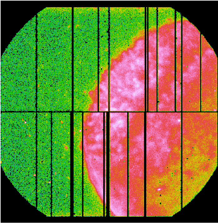
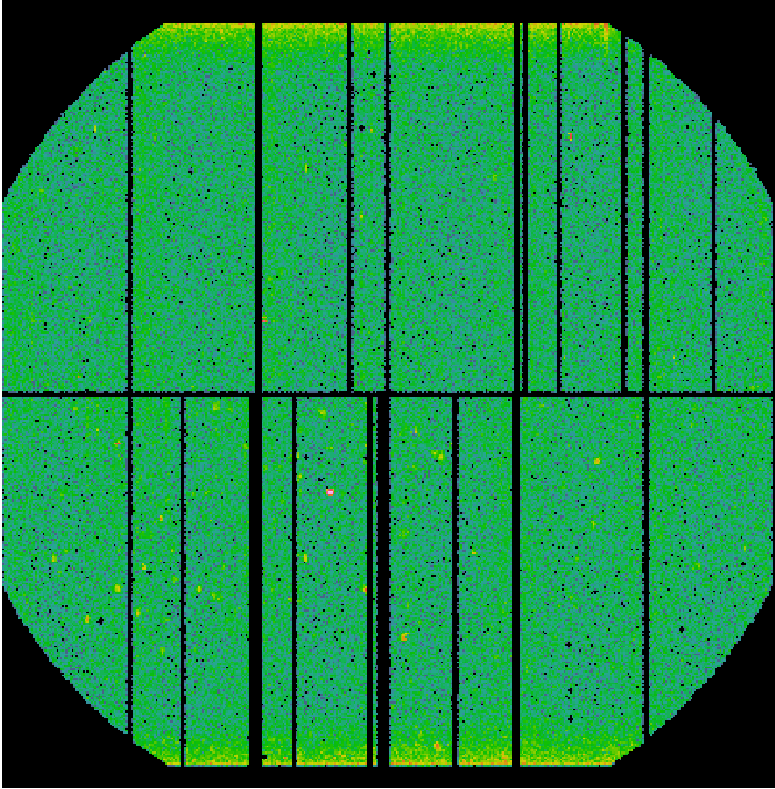
   Left panel: Science exposure (pn_sci_image.fit); Middle panel: FWC exposure (pn_qpb_image.fit). The image is scaled by the ratio of exposure times. Right panel: Science exposure subtracted from the QPB background (pn_sci_corr_image.fit).

How to use the FWC event files for spectra generation

1. For this exercise, the obsid 0693741001 corresponding to a point-like source will be used to better illustrate the procedure.
   
   For spectra extraction, identify the source and background extraction regions. From our example obsid, we identify the source and background regions as circular, defined by (see Fig.2):
   
     DETX_Src = 2489
     DETY_Src = -8404
     Radius_Src = 1200
   
     DETX_Bkg = -663
     DETY_Bkg = -8404
     Radius_Bkg = 1200
   
   Use the same source region to extract source spectra from both the Science and FWC exposure and the same background region to extract background spectra from both the Science and FWC exposure. Please, have a look at the "EPIC status of calibration and data analysis" document ( XMM-SOC-CAL-TN-0018) for the latest recommendations on how to select source and background regions. Also, the threads How to extract PN spectra of a point-like source and associated matrices and Extraction and correction of an X-ray light curve for a point-like source indicate how to define extraction regions.
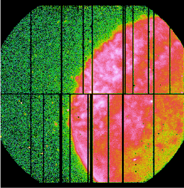
     Fig.2: Science and FWC EPIC-pn exposure images in detector coordinates (DETX,DETY) with Source (SRC) and Background (BKG) regions overlaid.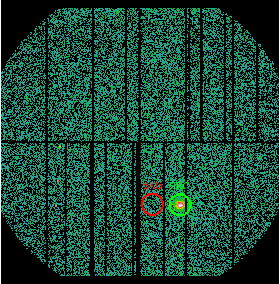
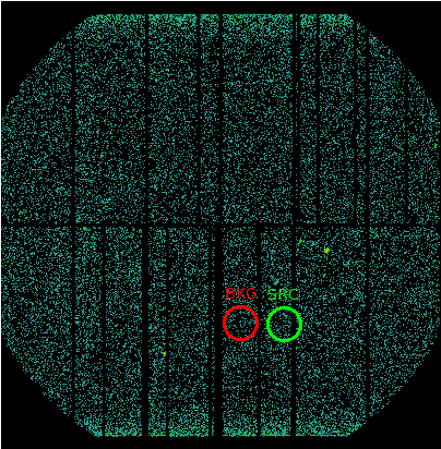
   Left panel: Science exposure (pn_sci_image.fit); Right panel: FWC exposure (pn_qpb_image.fit). The image is scaled by the ratio of exposure times.


2. Once the regions are identified for both source and background, a similar method to extract the spectra as that described in the thread Extraction of spectra in a few clicks: especget can be used to extract all the spectral products in one go from the science and FWC exposures. Otherwise, the thread How to extract PN spectra of a point-like source and associated matrices can also be followed to extract the different products, spectra and response files (arf, rmf), one by one. For this thread, the step that is important is the use of the same extraction regions on the science and FWC exposure, like in the example below:
   
        evselect table=pn_sci_clean.fits withspectrumset=yes spectrumset=PNsource_spectrum.fits \
       energycolumn=PI spectralbinsize=5 withspecranges=yes specchannelmin=0 specchannelmax=20479 \
       expression='(FLAG==0) && (PATTERN<=4) && ((DETX,DETY) IN circle(2489,-8404,1200))'
       ; for the source region of the science exposure
   
        evselect table=pn_qpb_clean.fits withspectrumset=yes spectrumset=PNsource_fwc_spectrum.fits \
       energycolumn=PI spectralbinsize=5 withspecranges=yes specchannelmin=0 specchannelmax=20479 \
       expression='(FLAG==0) && (PATTERN<=4) && ((DETX,DETY) IN circle(2489,-8404,1200))' \
       zcolumn='EWEIGHT'
       ; for the source region of the FWC exposure
   
        evselect table=pn_sci_clean.fits withspectrumset=yes spectrumset=PNbkg_spectrum.fits \
       energycolumn=PI spectralbinsize=5 withspecranges=yes specchannelmin=0 specchannelmax=20479 \
       expression='(FLAG==0) && (PATTERN<=4) && ((DETX,DETY) IN circle(-663,-8404,1200))'
       ; for the background region of the science exposure
   
        evselect table=pn_qpb_clean.fits withspectrumset=yes spectrumset=PNbkg_fwc_spectrum.fits \
       energycolumn=PI spectralbinsize=5 withspecranges=yes specchannelmin=0 specchannelmax=20479 \
       expression='(FLAG==0) && (PATTERN<=4) && ((DETX,DETY) IN circle(-663,-8404,1200))' \
       zcolumn='EWEIGHT'
       ; for the background region of the FWC exposure
   
   By using the zcolumn parameter in the generation of the spectra for the FWC exposure, we ensure that the produced FWC spectra are correctly scaled for the ratio of exposure times between science and FWC exposures. By doing so, the FWC spectra are ready to be subtracted from the science spectra.

    

3. To illustrate the validity of the method, Fig.3 shows as an example the comparisson of the average spectra extracted from the FWC (pink) and SN 1006-1 science (grey) exposures. The FWC exposure spectra has been extracted from the tailored exposure as provided by the task evqpb with the method described above. The top panel shows the average spectra of the out-of-field events. Both spectra should be identical and the ratio of one to the other should be equal to 1 across all energies (blue curve). However, the out-of-field data from the science exposure is contaminated by the SN 1006-1, hence at low energies the agreement is not as expected, but at high energies where there is no contribution from the SN 1006-1, the agreement is very good within a few percent. The bottom panel of this figure shows the same but for the in-field-of-view data. In this case the comparisson at low energies does not make sence because the science spectrum is dominated by the SN 1006-1. However at high energies, again, where there is no contribution from the source, the agreement is good within a few percent. The blue curve this time shows the science spectrum minus the FWC spectrum.

    

   Fig.3: Comparisson of the average spectra derived from the FWC (pink) and SN 1006-1 science (grey) exposures. The top pannel shows the average spectra of the out-of-field events, while the bottom panel shows the in-field-of-view events (see text for details).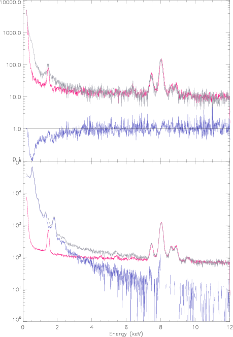

An Alternative method FOR deriving QPB products for EPIC-pN

As of SASv19, a new task has been introduced, qpbselect, to deal with the QPB in science exposures. qpbselect expands the functionality of evqpb by using the number of discarded lines (NDISCLIN) to estimate the level of the QPB affecting a given science EPIC-pn exposure. The task will produce a corresponding QPB event file, image and spectrum that can be used to correct the science data. This method is only valid for EPIC-pn, and as of SASv21, applicable only to FF andn EFF mode data. The steps to run this task are given below.

1. Set up your SAS environment (see Prerequisites for this thread at the top of the page).
    
2. Create an EPIC-pn event file for your science observation (see Prerequisites for this thread at the top of the page). The name of the event file that will be used in this thread is:
   
      2382_0690510101_EPN_S003_ImagingEvts.ds
   
   which contains events from a FF mode exposure within obsid 0690510101.
    
3. If necessary, filter the EPIC-pn event file to create a cleaned and filtered for flaring particle background event file for your observation (see Prerequisites for this thread at the top of the page). Let the name of the GTI filtered event file be, pn_sci_clean.fits
4. Create an image and a spectrum from this event file:
   1. Produce Image,
      
         evselect table=pn_sci_clean.fits \
             withimageset=yes imageset=PNimage.ds \
             imagebinning=binSize xcolumn=X ycolumn=Y ximagebinsize=80 yimagebinsize=80 \
             expression='Selection_Expression'
      
      where the Selection_Expression can take any desired form for the image to be produced, for example:
      
        #XMMEA_EP && (PATTERN<=4)
      
      in this example the output image file name is PNimage.ds.
       
   2. Produce Spectrum,
      
         evselect table=pn_sci_clean.fits \
             withspectrumset=yes spectrumset=PNsource_spectrum.fits \
             energycolumn=PI spectralbinsize=5 withspecranges=yes \ 
                      specchannelmin=0 specchannelmax=20479 \
             expression='Selection_Expression'
      
      where the Selection_Expression can take any desired form for the spectrum to be produced, including the extraction region, for example:
      
        (FLAG==0) && (PATTERN<=4) && ((X,Y) IN circle(34404.944,22460.5,1200))
      
      in this example the output spectral file name is PNsource_spectrum.fits.
      
5. Run the SAS task qpbselect over the event file to produce in two separate steps a correspoding QPB image and spectrum.
   ​​​​​​​
   1. Produce Image,
      
         qpbselect table=pn_sci_clean.fits attfile=2382_0690510101_AttHk.ds \
             productname=PNimage.ds outprod=QPBPN_image.ds
       

      it is necessary to pass to the task the attitude history file via the parameter attfile, in this example, 2382_0690510101_AttHk.ds that is produced when generating the event file. The task needs to make use of the attitude history file corresponding to the science observation to recast the FWC events in space to match those of the science observation. The task will use as input the science image generated in the previous steps, PNimage.ds, and will output the corresponding QPB image file, QPBPN_image.ds. The image QPBPN_image.ds has been scaled and recasted to the science exposure sky position. Also, the same filter expression used to select event applied to the science image has been applied to the QPB image. ​​​

   2. Produce Spectrum,
      
         qpbselect table=pn_sci_clean.fits attfile=2382_0690510101_AttHk.ds \
             productname=PNsource_spectrum.fits outprod=QPBPN_spectrum.ds
       

      in this call the task will use as input the science spectrum generated in the previous steps, PNsource_spectrum.fits, and will output the corresponding QPB spectral file, QPBPN_spectrum.ds. The spectrum has been scaled to match the science spectrum.

6. qpbselect also outputs the QPB event file used to generate the QPB image and spectrum, but keep in mind that this is the raw QPB event file used to produce the QPB image and spectrum, and has not been scaled to match the science data. However, the column EWEIGHT contains for every event the scaling factor that needs to be applied and can be used to produce further products from this file if needed.
   ​​​​​​​
7. Last, qpbselect adds a keyword to the QPB event file, image and spectrum containing the mean number of discarded lines (NDISCLIN) as derived for the science data over the good time intervals. The name of the keyword is DLMEAN.